Measure region properties

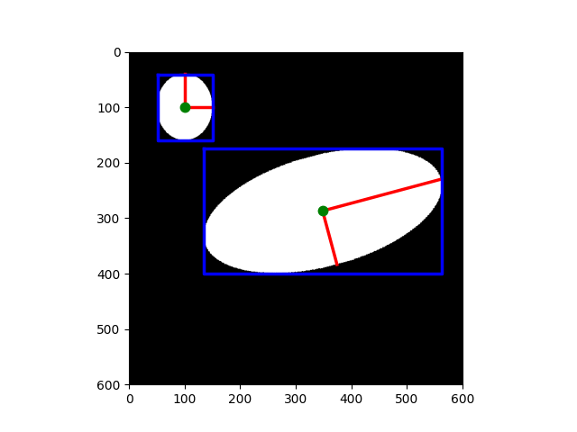
This example shows how to measure properties of labelled image regions. We first analyze an image with two ellipses. Below we show how to explore interactively the properties of labelled objects.

import math
import matplotlib.pyplot as plt
import numpy as np
import pandas as pd

from skimage.draw import ellipse
from skimage.measure import label, regionprops, regionprops_table
from skimage.transform import rotate


image = np.zeros((600, 600))

rr, cc = ellipse(300, 350, 100, 220)
image[rr, cc] = 1

image = rotate(image, angle=15, order=0)

rr, cc = ellipse(100, 100, 60, 50)
image[rr, cc] = 1

label_img = label(image)
regions = regionprops(label_img)

We use the skimage.measure.regionprops() result to draw certain properties on each region. For example, in red, we plot the major and minor axes of each ellipse.

fig, ax = plt.subplots()
ax.imshow(image, cmap=plt.cm.gray)

for props in regions:
    y0, x0 = props.centroid
    orientation = props.orientation
    x1 = x0 + math.cos(orientation) * 0.5 * props.axis_minor_length
    y1 = y0 - math.sin(orientation) * 0.5 * props.axis_minor_length
    x2 = x0 - math.sin(orientation) * 0.5 * props.axis_major_length
    y2 = y0 - math.cos(orientation) * 0.5 * props.axis_major_length

    ax.plot((x0, x1), (y0, y1), '-r', linewidth=2.5)
    ax.plot((x0, x2), (y0, y2), '-r', linewidth=2.5)
    ax.plot(x0, y0, '.g', markersize=15)

    minr, minc, maxr, maxc = props.bbox
    bx = (minc, maxc, maxc, minc, minc)
    by = (minr, minr, maxr, maxr, minr)
    ax.plot(bx, by, '-b', linewidth=2.5)

ax.axis((0, 600, 600, 0))
plt.show()

We use the skimage.measure.regionprops_table() function to compute (selected) properties for each region. Note that skimage.measure.regionprops_table actually computes the properties, whereas skimage.measure.regionprops computes them when they come in use (lazy evaluation).

props = regionprops_table(
    label_img,
    properties=('centroid', 'orientation', 'axis_major_length', 'axis_minor_length'),
)

We now display a table of these selected properties (one region per row), the skimage.measure.regionprops_table result being a pandas-compatible dict.

pd.DataFrame(props)

	centroid-0	centroid-1	orientation	axis_major_length	axis_minor_length
0	100.000000	100.000000	0.000000	119.807049	99.823995
1	286.914167	348.412995	-1.308966	440.015503	199.918850

It is also possible to explore interactively the properties of labelled objects by visualizing them in the hover information of the labels. This example uses plotly in order to display properties when hovering over the objects.

import plotly
import plotly.express as px
import plotly.graph_objects as go
from skimage import data, filters, measure, morphology

img = data.coins()
# Binary image, post-process the binary mask and compute labels
threshold = filters.threshold_otsu(img)
mask = img > threshold
mask = morphology.remove_small_objects(mask, 50)
mask = morphology.remove_small_holes(mask, 50)
labels = measure.label(mask)

fig = px.imshow(img, binary_string=True)
fig.update_traces(hoverinfo='skip')  # hover is only for label info

props = measure.regionprops(labels, img)
properties = ['area', 'eccentricity', 'perimeter', 'intensity_mean']

# For each label, add a filled scatter trace for its contour,
# and display the properties of the label in the hover of this trace.
for index in range(1, labels.max()):
    label_i = props[index].label
    contour = measure.find_contours(labels == label_i, 0.5)[0]
    y, x = contour.T
    hoverinfo = ''
    for prop_name in properties:
        hoverinfo += f'<b>{prop_name}: {getattr(props[index], prop_name):.2f}</b><br>'
    fig.add_trace(
        go.Scatter(
            x=x,
            y=y,
            name=label_i,
            mode='lines',
            fill='toself',
            showlegend=False,
            hovertemplate=hoverinfo,
            hoveron='points+fills',
        )
    )

plotly.io.show(fig)