Using geometric transformations

In this example, we will see how to use geometric transformations in the context of image processing.

import math
import numpy as np
import matplotlib.pyplot as plt

from skimage import data
from skimage import transform

Basics

Several different geometric transformation types are supported: similarity, affine, projective and polynomial. For a tutorial on the available types of transformations, see Types of homographies.

Geometric transformations can either be created using the explicit parameters (e.g. scale, shear, rotation and translation) or the transformation matrix.

First we create a transformation using explicit parameters:

tform = transform.SimilarityTransform(scale=1, rotation=math.pi / 2, translation=(0, 1))
print(tform.params)

[[ 6.123234e-17 -1.000000e+00  0.000000e+00]
 [ 1.000000e+00  6.123234e-17  1.000000e+00]
 [ 0.000000e+00  0.000000e+00  1.000000e+00]]

Alternatively you can define a transformation by the transformation matrix itself:

matrix = tform.params.copy()
matrix[1, 2] = 2
tform2 = transform.SimilarityTransform(matrix)

These transformation objects can then be used to apply forward and inverse coordinate transformations between the source and destination coordinate systems:

coord = [1, 0]
print(tform2(coord))
print(tform2.inverse(tform(coord)))

[[6.123234e-17 3.000000e+00]]
[[ 0.000000e+00 -6.123234e-17]]

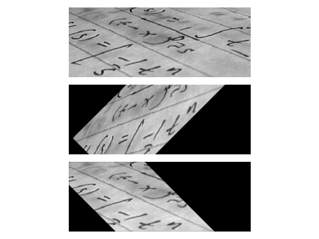
Image warping

Geometric transformations can also be used to warp images:

text = data.text()

tform = transform.SimilarityTransform(
    scale=1, rotation=math.pi / 4, translation=(text.shape[0] / 2, -100)
)

rotated = transform.warp(text, tform)
back_rotated = transform.warp(rotated, tform.inverse)

fig, ax = plt.subplots(nrows=3)

ax[0].imshow(text, cmap=plt.cm.gray)
ax[1].imshow(rotated, cmap=plt.cm.gray)
ax[2].imshow(back_rotated, cmap=plt.cm.gray)

for a in ax:
    a.axis('off')

plt.tight_layout()

Parameter estimation

In addition to the basic functionality mentioned above you can also estimate the parameters of a geometric transformation using the least- squares method.

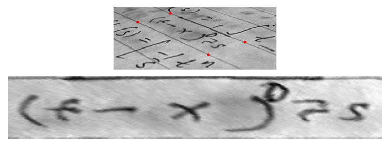
This can amongst other things be used for image registration or rectification, where you have a set of control points or homologous/corresponding points in two images.

Let’s assume we want to recognize letters on a photograph which was not taken from the front but at a certain angle. In the simplest case of a plane paper surface the letters are projectively distorted. Simple matching algorithms would not be able to match such symbols. One solution to this problem would be to warp the image so that the distortion is removed and then apply a matching algorithm:

text = data.text()

src = np.array([[0, 0], [0, 50], [300, 50], [300, 0]])
dst = np.array([[155, 15], [65, 40], [260, 130], [360, 95]])

tform3 = transform.ProjectiveTransform()
tform3.estimate(src, dst)
warped = transform.warp(text, tform3, output_shape=(50, 300))

fig, ax = plt.subplots(nrows=2, figsize=(8, 3))

ax[0].imshow(text, cmap=plt.cm.gray)
ax[0].plot(dst[:, 0], dst[:, 1], '.r')
ax[1].imshow(warped, cmap=plt.cm.gray)

for a in ax:
    a.axis('off')

plt.tight_layout()
plt.show()

The above estimation relies on accurate knowledge of the location of points and an accurate selection of their correspondence. If point locations have an uncertainty associated with them, then weighting can be provided so that the resulting transform prioritises an accurate fit to those points with the highest weighting. An alternative approach called the RANSAC algorithm is useful when the correspondence points are not perfectly accurate. See the Robust matching using RANSAC tutorial for an in-depth description of how to use this approach in scikit-image.