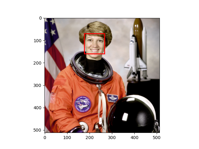
Face detection using a cascade classifier

This computer vision example shows how to detect faces on an image using object detection framework based on machine learning.

First, you will need an xml file, from which the trained data can be read. The framework works with files, trained using Multi-block Local Binary Patterns Features (See MB-LBP) and Gentle Adaboost with attentional cascade. So, the detection framework will also work with xml files from OpenCV. There you can find files that were trained to detect cat faces, profile faces and other things. But if you want to detect frontal faces, the respective file is already included in scikit-image.

Next you will have to specify the parameters for the detect_multi_scale function. Here you can find the meaning of each of them.

First one is scale_ratio. To find all faces, the algorithm does the search on multiple scales. This is done by changing the size of searching window. The smallest window size is the size of window that was used in training. This size is specified in the xml file with trained parameters. The scale_ratio parameter specifies by which ratio the search window is increased on each step. If you increase this parameter, the search time decreases and the accuracy decreases. So, faces on some scales can be not detected.

step_ratio specifies the step of sliding window that is used to search for faces on each scale of the image. If this parameter is equal to one, then all the possible locations are searched. If the parameter is greater than one, for example, two, the window will be moved by two pixels and not all of the possible locations will be searched for faces. By increasing this parameter we can reduce the working time of the algorithm, but the accuracy will also be decreased.

min_size is the minimum size of search window during the scale search. max_size specifies the maximum size of the window. If you know the size of faces on the images that you want to search, you should specify these parameters as precisely as possible, because you can avoid doing expensive computations and possibly decrease the amount of false detections. You can save a lot of time by increasing the min_size parameter, because the majority of time is spent on searching on the smallest scales.

min_neighbor_number and intersection_score_threshold parameters are made to cluster the excessive detections of the same face and to filter out false detections. True faces usually have a lot of detections around them and false ones usually have single detection. First algorithm searches for clusters: two rectangle detections are placed in the same cluster if the intersection score between them is larger then intersection_score_threshold. The intersection score is computed using the equation (intersection area) / (small rectangle ratio). The described intersection criteria was chosen over intersection over union to avoid a corner case when small rectangle inside of a big one has small intersection score. Then each cluster is thresholded using min_neighbor_number parameter which leaves the clusters that have a same or bigger number of detections in them.

You should also take into account that false detections are inevitable and if you want to have a really precise detector, you will have to train it yourself using OpenCV train cascade utility.

from skimage import data
from skimage.feature import Cascade

import matplotlib.pyplot as plt
from matplotlib import patches

# Load the trained file from the module root.
trained_file = data.lbp_frontal_face_cascade_filename()

# Initialize the detector cascade.
detector = Cascade(trained_file)

img = data.astronaut()

detected = detector.detect_multi_scale(
    img=img, scale_factor=1.2, step_ratio=1, min_size=(60, 60), max_size=(123, 123)
)

fig, ax = plt.subplots()
ax.imshow(img, cmap='gray')

for patch in detected:
    ax.axes.add_patch(
        patches.Rectangle(
            (patch['c'], patch['r']),
            patch['width'],
            patch['height'],
            fill=False,
            color='r',
            linewidth=2,
        )
    )

plt.show()