Registration using optical flow

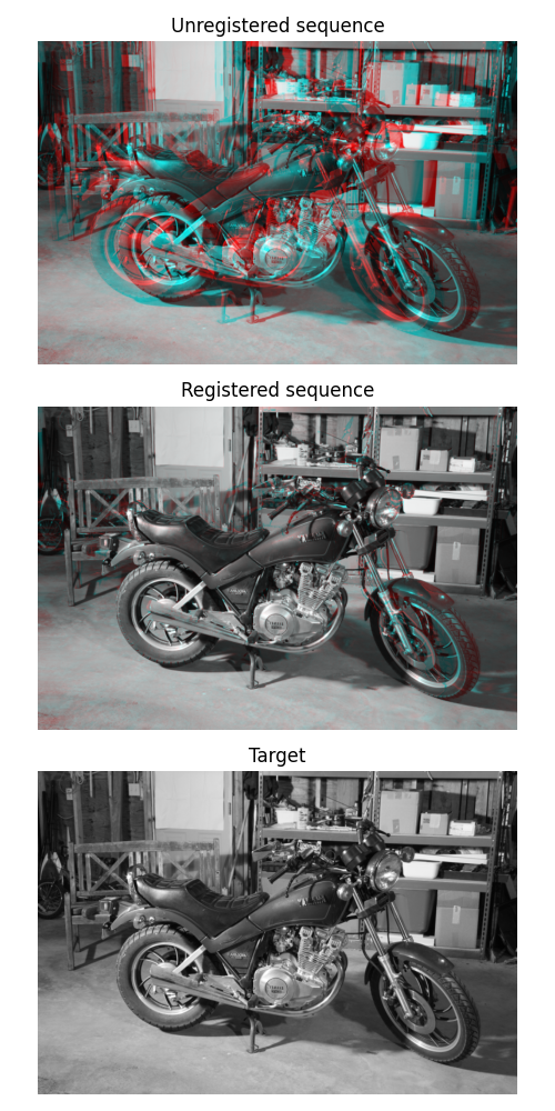
Demonstration of image registration using optical flow.

By definition, the optical flow is the vector field (u, v) verifying image1(x+u, y+v) = image0(x, y), where (image0, image1) is a couple of consecutive 2D frames from a sequence. This vector field can then be used for registration by image warping.

To display registration results, an RGB image is constructed by assigning the result of the registration to the red channel and the target image to the green and blue channels. A perfect registration results in a gray level image while misregistred pixels appear colored in the constructed RGB image.

import numpy as np
from matplotlib import pyplot as plt
from skimage.color import rgb2gray
from skimage.data import stereo_motorcycle, vortex
from skimage.transform import warp
from skimage.registration import optical_flow_tvl1, optical_flow_ilk

# --- Load the sequence
image0, image1, disp = stereo_motorcycle()

# --- Convert the images to gray level: color is not supported.
image0 = rgb2gray(image0)
image1 = rgb2gray(image1)

# --- Compute the optical flow
v, u = optical_flow_tvl1(image0, image1)

# --- Use the estimated optical flow for registration

nr, nc = image0.shape

row_coords, col_coords = np.meshgrid(np.arange(nr), np.arange(nc), indexing='ij')

image1_warp = warp(image1, np.array([row_coords + v, col_coords + u]), mode='edge')

# build an RGB image with the unregistered sequence
seq_im = np.zeros((nr, nc, 3))
seq_im[..., 0] = image1
seq_im[..., 1] = image0
seq_im[..., 2] = image0

# build an RGB image with the registered sequence
reg_im = np.zeros((nr, nc, 3))
reg_im[..., 0] = image1_warp
reg_im[..., 1] = image0
reg_im[..., 2] = image0

# build an RGB image with the registered sequence
target_im = np.zeros((nr, nc, 3))
target_im[..., 0] = image0
target_im[..., 1] = image0
target_im[..., 2] = image0

# --- Show the result

fig, (ax0, ax1, ax2) = plt.subplots(3, 1, figsize=(5, 10))

ax0.imshow(seq_im)
ax0.set_title("Unregistered sequence")
ax0.set_axis_off()

ax1.imshow(reg_im)
ax1.set_title("Registered sequence")
ax1.set_axis_off()

ax2.imshow(target_im)
ax2.set_title("Target")
ax2.set_axis_off()

fig.tight_layout()

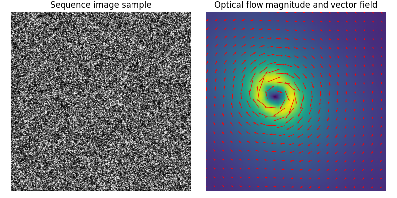
The estimated vector field (u, v) can also be displayed with a quiver plot.

In the following example, Iterative Lukas-Kanade algorithm (iLK) is applied to images of particles in the context of particle image velocimetry (PIV). The sequence is the Case B from the PIV challenge 2001

image0, image1 = vortex()

# --- Compute the optical flow
v, u = optical_flow_ilk(image0, image1, radius=15)

# --- Compute flow magnitude
norm = np.sqrt(u**2 + v**2)

# --- Display
fig, (ax0, ax1) = plt.subplots(1, 2, figsize=(8, 4))

# --- Sequence image sample

ax0.imshow(image0, cmap='gray')
ax0.set_title("Sequence image sample")
ax0.set_axis_off()

# --- Quiver plot arguments

nvec = 20  # Number of vectors to be displayed along each image dimension
nl, nc = image0.shape
step = max(nl // nvec, nc // nvec)

y, x = np.mgrid[:nl:step, :nc:step]
u_ = u[::step, ::step]
v_ = v[::step, ::step]

ax1.imshow(norm)
ax1.quiver(x, y, u_, v_, color='r', units='dots', angles='xy', scale_units='xy', lw=3)
ax1.set_title("Optical flow magnitude and vector field")
ax1.set_axis_off()
fig.tight_layout()

plt.show()