Note

Go to the end to download the full example code. or to run this example in your browser via Binder

Segment human cells (in mitosis)#

In this example, we analyze a microscopy image of human cells. We use data provided by Jason Moffat [1] through CellProfiler.

import matplotlib.pyplot as plt
import numpy as np
from scipy import ndimage as ndi

import skimage as ski

image = ski.data.human_mitosis()

fig, ax = plt.subplots()
ax.imshow(image, cmap='gray')
ax.set_title('Microscopy image of human cells stained for nuclear DNA')
plt.show()

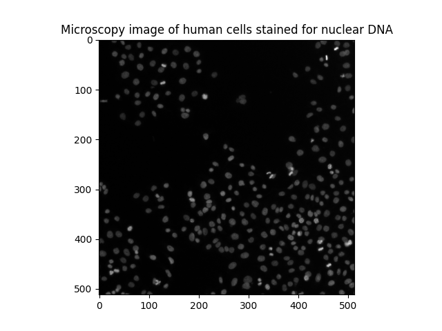
Microscopy image of human cells stained for nuclear DNA

We can see many cell nuclei on a dark background. Most of them are smooth and have an elliptical shape. However, we can distinguish some brighter spots corresponding to nuclei undergoing mitosis (cell division).

Another way of visualizing a grayscale image is contour plotting:

fig, ax = plt.subplots(figsize=(5, 5))
qcs = ax.contour(image, origin='image')
ax.set_title('Contour plot of the same raw image')
plt.show()

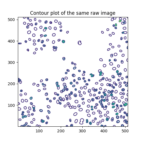
The contour lines are drawn at these levels:

qcs.levels

array([  0.,  40.,  80., 120., 160., 200., 240., 280.])

Each level has, respectively, the following number of segments:

# Levels without segments still contain one empty array, account for that
[len(seg) if seg[0].size else 0 for seg in qcs.allsegs]

[0, 320, 270, 48, 19, 3, 1, 0]

Estimate the mitotic index#

Cell biology uses the mitotic index to quantify cell division and, hence, cell proliferation. By definition, it is the ratio of cells in mitosis over the total number of cells. To analyze the above image, we are thus interested in two thresholds: one separating the nuclei from the background, the other separating the dividing nuclei (brighter spots) from the non-dividing nuclei. To separate these three different classes of pixels, we resort to Multi-Otsu Thresholding.

thresholds = ski.filters.threshold_multiotsu(image, classes=3)
regions = np.digitize(image, bins=thresholds)

fig, ax = plt.subplots(ncols=2, figsize=(10, 5))
ax[0].imshow(image)
ax[0].set_title('Original')
ax[0].set_axis_off()
ax[1].imshow(regions)
ax[1].set_title('Multi-Otsu thresholding')
ax[1].set_axis_off()
plt.show()

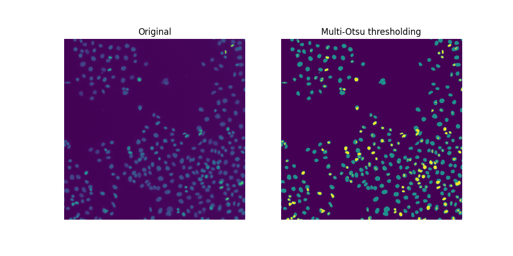
Since there are overlapping nuclei, thresholding is not enough to segment all the nuclei. If it were, we could readily compute a mitotic index for this sample:

cells = image > thresholds[0]
dividing = image > thresholds[1]
labeled_cells = ski.measure.label(cells)
labeled_dividing = ski.measure.label(dividing)
naive_mi = labeled_dividing.max() / labeled_cells.max()
print(naive_mi)

0.7847222222222222

Whoa, this can’t be! The number of dividing nuclei

print(labeled_dividing.max())

is overestimated, while the total number of cells

print(labeled_cells.max())

is underestimated.

fig, ax = plt.subplots(ncols=3, figsize=(15, 5))
ax[0].imshow(image)
ax[0].set_title('Original')
ax[0].set_axis_off()
ax[1].imshow(dividing)
ax[1].set_title('Dividing nuclei?')
ax[1].set_axis_off()
ax[2].imshow(cells)
ax[2].set_title('All nuclei?')
ax[2].set_axis_off()
plt.show()

Count dividing nuclei#

Clearly, not all connected regions in the middle plot are dividing nuclei. On one hand, the second threshold (value of thresholds[1]) appears to be too low to separate those very bright areas corresponding to dividing nuclei from relatively bright pixels otherwise present in many nuclei. On the other hand, we want a smoother image, removing small spurious objects and, possibly, merging clusters of neighboring objects (some could correspond to two nuclei emerging from one cell division). In a way, the segmentation challenge we are facing with dividing nuclei is the opposite of that with (touching) cells.

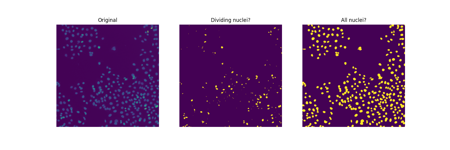
To find suitable values for thresholds and filtering parameters, we proceed by dichotomy, visually and manually.

higher_threshold = 125
dividing = image > higher_threshold

smoother_dividing = ski.filters.rank.mean(
    ski.util.img_as_ubyte(dividing), ski.morphology.disk(4)
)

binary_smoother_dividing = smoother_dividing > 20

fig, ax = plt.subplots(figsize=(5, 5))
ax.imshow(binary_smoother_dividing)
ax.set_title('Dividing nuclei')
ax.set_axis_off()
plt.show()

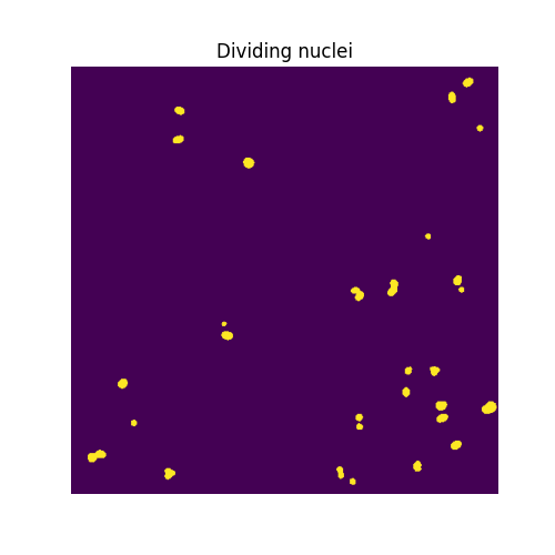
We are left with

cleaned_dividing = ski.measure.label(binary_smoother_dividing)
print(cleaned_dividing.max())

dividing nuclei in this sample.

Segment nuclei#

To separate overlapping nuclei, we resort to Watershed segmentation. The idea of the algorithm is to find watershed basins as if flooded from a set of markers. We generate these markers as the local maxima of the distance function to the background. Given the typical size of the nuclei, we pass min_distance=7 so that local maxima and, hence, markers will lie at least 7 pixels away from one another. We also use exclude_border=False so that all nuclei touching the image border will be included.

distance = ndi.distance_transform_edt(cells)

local_max_coords = ski.feature.peak_local_max(
    distance, min_distance=7, exclude_border=False
)
local_max_mask = np.zeros(distance.shape, dtype=bool)
local_max_mask[tuple(local_max_coords.T)] = True
markers = ski.measure.label(local_max_mask)

segmented_cells = ski.segmentation.watershed(-distance, markers, mask=cells)

To visualize the segmentation conveniently, we colour-code the labelled regions using the color.label2rgb function, specifying the background label with argument bg_label=0.

fig, ax = plt.subplots(ncols=2, figsize=(10, 5))
ax[0].imshow(cells, cmap='gray')
ax[0].set_title('Overlapping nuclei')
ax[0].set_axis_off()
ax[1].imshow(ski.color.label2rgb(segmented_cells, bg_label=0))
ax[1].set_title('Segmented nuclei')
ax[1].set_axis_off()
plt.show()

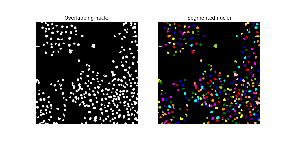
Make sure that the watershed algorithm has led to identifying more nuclei:

assert segmented_cells.max() > labeled_cells.max()

Finally, we find a total number of

print(segmented_cells.max())

cells in this sample. Therefore, we estimate the mitotic index to be:

print(cleaned_dividing.max() / segmented_cells.max())

0.0914826498422713

Total running time of the script: (0 minutes 3.625 seconds)

Gallery generated by Sphinx-Gallery