Interact with 3D images (of kidney tissue)

In this tutorial, we explore interactively a biomedical image which has three spatial dimensions and three color dimensions (channels). For a general introduction to 3D image processing, please refer to Explore 3D images (of cells). The data we use here correspond to kidney tissue which was imaged with confocal fluorescence microscopy (more details at [1] under kidney-tissue-fluorescence.tif).

[1]

scikit-image/data/#data

import matplotlib.pyplot as plt
import numpy as np

import plotly
import plotly.express as px
from skimage import data

Load image

This biomedical image is available through scikit-image’s data registry.

data = data.kidney()

The returned dataset is a 3D multichannel image:

print(f'number of dimensions: {data.ndim}')
print(f'shape: {data.shape}')
print(f'dtype: {data.dtype}')

number of dimensions: 4
shape: (16, 512, 512, 3)
dtype: uint16

Dimensions are provided in the following order: (z, y, x, c), i.e., [plane, row, column, channel].

n_plane, n_row, n_col, n_chan = data.shape

Let us consider only a slice (2D plane) of the data for now. More specifically, let us consider the slice located halfway in the stack. The imshow function can display both grayscale and RGB(A) 2D images.

_, ax = plt.subplots()
ax.imshow(data[n_plane // 2])

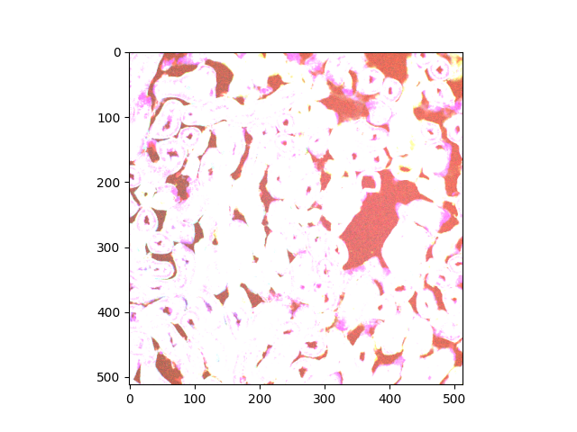
Clipping input data to the valid range for imshow with RGB data ([0..1] for floats or [0..255] for integers).

<matplotlib.image.AxesImage object at 0x7fe84e5f82c0>

According to the warning message, the range of values is unexpected. The image rendering is clearly not satisfactory color-wise.

vmin, vmax = data.min(), data.max()
print(f'range: ({vmin}, {vmax})')

range: (10, 4095)

We turn to Plotly’s implementation of the plotly.express.imshow() function, for it supports value ranges beyond (0.0, 1.0) for floats and (0, 255) for integers.

fig = px.imshow(data[n_plane // 2], zmax=vmax)
plotly.io.show(fig)

Here you go, fluorescence microscopy!

Normalize range for each channel

Generally speaking, we may want to normalize the value range on a per-channel basis. Let us facet our data (slice) along the channel axis. This way, we get three single-channel images, where the max value of each image is used:

fig = px.imshow(
    data[n_plane // 2], facet_col=2, binary_string=True, labels={'facet_col': 'channel'}
)
plotly.io.show(fig)

What is the range of values for each color channel? We check by taking the min and max across all non-channel axes.

vmin_0, vmin_1, vmin_2 = np.min(data, axis=(0, 1, 2))
vmax_0, vmax_1, vmax_2 = np.max(data, axis=(0, 1, 2))
print(f'range for channel 0: ({vmin_0}, {vmax_0})')
print(f'range for channel 1: ({vmin_1}, {vmax_1})')
print(f'range for channel 2: ({vmin_2}, {vmax_2})')

range for channel 0: (10, 4095)
range for channel 1: (68, 4095)
range for channel 2: (35, 4095)

Let us be very specific and pass value ranges on a per-channel basis:

fig = px.imshow(
    data[n_plane // 2], zmin=[vmin_0, vmin_1, vmin_2], zmax=[vmax_0, vmax_1, vmax_2]
)
plotly.io.show(fig)

Plotly lets you interact with this visualization by panning, zooming in and out, and exporting the desired figure as a static image in PNG format.

Explore slices as animation frames

Click the play button to move along the z axis, through the stack of all 16 slices.

fig = px.imshow(
    data,
    zmin=[vmin_0, vmin_1, vmin_2],
    zmax=[vmax_0, vmax_1, vmax_2],
    animation_frame=0,
    binary_string=True,
    labels={'animation_frame': 'plane'},
)
plotly.io.show(fig)

Combine channel facetting and slice animation

fig = px.imshow(
    data,
    animation_frame=0,
    facet_col=3,
    binary_string=True,
    labels={'facet_col': 'channel', 'animation_frame': 'plane'},
)
plotly.io.show(fig)

The biologist’s eye can spot that the two bright blobs (best seen in channel=2) are kidney glomeruli [2].

[2]

https://en.wikipedia.org/wiki/Glomerulus_(kidney)

plt.show()