Note
Go to the end to download the full example code or to run this example in your browser via Binder.
Use thin-plate splines for image warping#
To warp an image, we start with a set of source and target coordinates. The goal is to deform the image such that the source points move to the target locations. Typically, we only know the target positions for a few, select source points. To calculate the target positions for all other pixel positions, we need a model. Various such models exist, such as affine or projective transformations.
Most transformations are linear (i.e., they preserve straight lines), but sometimes we need more flexibility. One model that represents a non-linear transformation, i.e. one where lines can bend, is thin-plate splines [1] [2].
Thin-plate splines draw on the analogy of a metal sheet, which has inherent rigidity. Consider our source points: each has to move a certain distance, in both the x and y directions, to land in its corresponding target position. First, examine only the x coordinates. Imagine placing a thin metal plate on top of the image. Now bend it, such that at each source point, the plate’s z offset is the distance, positive or negative, that that source point has to travel in the x direction in order to land in its target position. The plate resists bending, and therefore remains smooth. We can read offsets for coordinates other than source points from the position of the plate. The same procedure can be repeated for the y coordinates.
This gives us our thin-plate spline model that maps any (x, y) coordinate to a target position.
Correct barrel distortion#
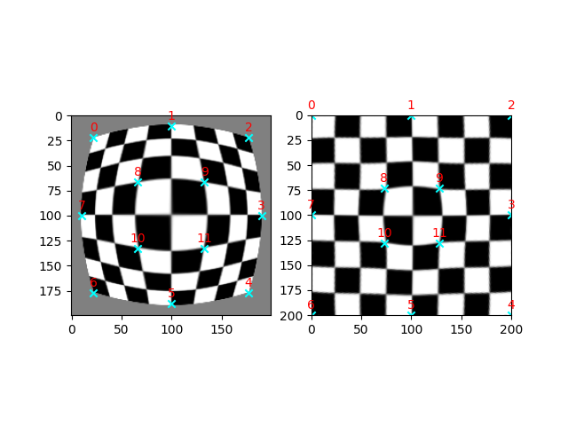
In this example, we demonstrate how to correct barrel distortion [3] using a thin-plate spline transform. Barrel distortion creates the characteristic fisheye effect, where image magnification decreases with distance from the image center.
We first generate an example dataset, by applying a fisheye warp to a checkboard image, and thereafter apply the inverse corrective transform.
https://en.wikipedia.org/wiki/Distortion_(optics)#Radial_distortion

import matplotlib.pyplot as plt
import numpy as np

import skimage as ski


def radial_distortion(xy, k1=0.9, k2=0.5):
    """Distort coordinates `xy` symmetrically around their own center."""
    xy_c = xy.max(axis=0) / 2
    xy = (xy - xy_c) / xy_c
    radius = np.linalg.norm(xy, axis=1)
    distortion_model = (1 + k1 * radius + k2 * radius**2) * k2
    xy *= distortion_model.reshape(-1, 1)
    xy = xy * xy_c + xy_c
    return xy


image = ski.data.checkerboard()
image = ski.transform.warp(image, radial_distortion, cval=0.5)


# Pick a few `src` points by hand, and move the corresponding `dst` points to their
# expected positions.
# fmt: off
src = np.array([[22,  22], [100,  10], [177, 22], [190, 100], [177, 177], [100, 188],
                [22, 177], [ 10, 100], [ 66, 66], [133,  66], [ 66, 133], [133, 133]])
dst = np.array([[ 0,   0], [100,   0], [200,  0], [200, 100], [200, 200], [100, 200],
                [ 0, 200], [  0, 100], [ 73, 73], [128,  73], [ 73, 128], [128, 128]])
# fmt: on

# Estimate the TPS transformation from these points and then warp the image.
# We switch `src` and `dst` here because `skimage.transform.warp` requires the
# inverse transformation!
tps = ski.transform.ThinPlateSplineTransform.from_estimate(dst, src)
warped = ski.transform.warp(image, tps)


# Plot the results
fig, axs = plt.subplots(1, 2)
axs[0].imshow(image, cmap='gray')
axs[0].scatter(src[:, 0], src[:, 1], marker='x', color='cyan')
axs[1].imshow(warped, cmap='gray', extent=(0, 200, 200, 0))
axs[1].scatter(dst[:, 0], dst[:, 1], marker='x', color='cyan')

point_labels = [str(i) for i in range(len(src))]
for i, label in enumerate(point_labels):
    axs[0].annotate(
        label,
        (src[:, 0][i], src[:, 1][i]),
        textcoords="offset points",
        xytext=(0, 5),
        ha='center',
        color='red',
    )
    axs[1].annotate(
        label,
        (dst[:, 0][i], dst[:, 1][i]),
        textcoords="offset points",
        xytext=(0, 5),
        ha='center',
        color='red',
    )

plt.show()
Total running time of the script: (0 minutes 0.265 seconds)
