Evaluating segmentation metrics

When trying out different segmentation methods, how do you know which one is best? If you have a ground truth or gold standard segmentation, you can use various metrics to check how close each automated method comes to the truth. In this example we use an easy-to-segment image as an example of how to interpret various segmentation metrics. We will use the adapted Rand error and the variation of information as example metrics, and see how oversegmentation (splitting of true segments into too many sub-segments) and undersegmentation (merging of different true segments into a single segment) affect the different scores.

import numpy as np
import matplotlib.pyplot as plt
from scipy import ndimage as ndi

from skimage import data
from skimage.metrics import adapted_rand_error, variation_of_information
from skimage.filters import sobel
from skimage.measure import label
from skimage.util import img_as_float
from skimage.feature import canny
from skimage.morphology import remove_small_objects
from skimage.segmentation import (
    morphological_geodesic_active_contour,
    inverse_gaussian_gradient,
    watershed,
    mark_boundaries,
)

image = data.coins()

First, we generate the true segmentation. For this simple image, we know exact functions and parameters that will produce a perfect segmentation. In a real scenario, typically you would generate ground truth by manual annotation or “painting” of a segmentation.

elevation_map = sobel(image)
markers = np.zeros_like(image)
markers[image < 30] = 1
markers[image > 150] = 2
im_true = watershed(elevation_map, markers)
im_true = ndi.label(ndi.binary_fill_holes(im_true - 1))[0]

Next, we create three different segmentations with different characteristics. The first one uses skimage.segmentation.watershed() with compactness, which is a useful initial segmentation but too fine as a final result. We will see how this causes the oversegmentation metrics to shoot up.

edges = sobel(image)
im_test1 = watershed(edges, markers=468, compactness=0.001)

The next approach uses the Canny edge filter, skimage.feature.canny(). This is a very good edge finder, and gives balanced results.

edges = canny(image)
fill_coins = ndi.binary_fill_holes(edges)
im_test2 = ndi.label(remove_small_objects(fill_coins, 21))[0]

Finally, we use morphological geodesic active contours, skimage.segmentation.morphological_geodesic_active_contour(), a method that generally produces good results, but requires a long time to converge on a good answer. We purposefully cut short the procedure at 100 iterations, so that the final result is undersegmented, meaning that many regions are merged into one segment. We will see the corresponding effect on the segmentation metrics.

image = img_as_float(image)
gradient = inverse_gaussian_gradient(image)
init_ls = np.zeros(image.shape, dtype=np.int8)
init_ls[10:-10, 10:-10] = 1
im_test3 = morphological_geodesic_active_contour(
    gradient,
    num_iter=100,
    init_level_set=init_ls,
    smoothing=1,
    balloon=-1,
    threshold=0.69,
)
im_test3 = label(im_test3)

method_names = [
    'Compact watershed',
    'Canny filter',
    'Morphological Geodesic Active Contours',
]
short_method_names = ['Compact WS', 'Canny', 'GAC']

precision_list = []
recall_list = []
split_list = []
merge_list = []
for name, im_test in zip(method_names, [im_test1, im_test2, im_test3]):
    error, precision, recall = adapted_rand_error(im_true, im_test)
    splits, merges = variation_of_information(im_true, im_test)
    split_list.append(splits)
    merge_list.append(merges)
    precision_list.append(precision)
    recall_list.append(recall)
    print(f'\n## Method: {name}')
    print(f'Adapted Rand error: {error}')
    print(f'Adapted Rand precision: {precision}')
    print(f'Adapted Rand recall: {recall}')
    print(f'False Splits: {splits}')
    print(f'False Merges: {merges}')

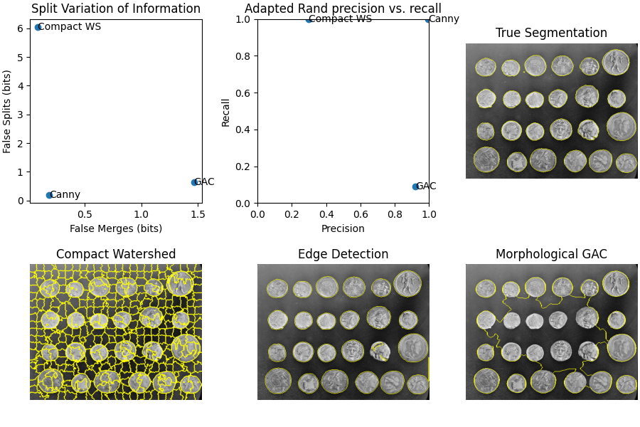
fig, axes = plt.subplots(2, 3, figsize=(9, 6), constrained_layout=True)
ax = axes.ravel()

ax[0].scatter(merge_list, split_list)
for i, txt in enumerate(short_method_names):
    ax[0].annotate(txt, (merge_list[i], split_list[i]), verticalalignment='center')
ax[0].set_xlabel('False Merges (bits)')
ax[0].set_ylabel('False Splits (bits)')
ax[0].set_title('Split Variation of Information')

ax[1].scatter(precision_list, recall_list)
for i, txt in enumerate(short_method_names):
    ax[1].annotate(txt, (precision_list[i], recall_list[i]), verticalalignment='center')
ax[1].set_xlabel('Precision')
ax[1].set_ylabel('Recall')
ax[1].set_title('Adapted Rand precision vs. recall')
ax[1].set_xlim(0, 1)
ax[1].set_ylim(0, 1)

ax[2].imshow(mark_boundaries(image, im_true))
ax[2].set_title('True Segmentation')
ax[2].set_axis_off()

ax[3].imshow(mark_boundaries(image, im_test1))
ax[3].set_title('Compact Watershed')
ax[3].set_axis_off()

ax[4].imshow(mark_boundaries(image, im_test2))
ax[4].set_title('Edge Detection')
ax[4].set_axis_off()

ax[5].imshow(mark_boundaries(image, im_test3))
ax[5].set_title('Morphological GAC')
ax[5].set_axis_off()

plt.show()

## Method: Compact watershed
Adapted Rand error: 0.5421684624091794
Adapted Rand precision: 0.2968781380256405
Adapted Rand recall: 0.9999664222191392
False Splits: 6.036024332525564
False Merges: 0.0825883711820654

## Method: Canny filter
Adapted Rand error: 0.0027247598212836177
Adapted Rand precision: 0.9946425605360896
Adapted Rand recall: 0.9999218934767155
False Splits: 0.20042002116129515
False Merges: 0.18076872508600775

## Method: Morphological Geodesic Active Contours
Adapted Rand error: 0.8346015951433162
Adapted Rand precision: 0.9191321393095933
Adapted Rand recall: 0.09087577915161697
False Splits: 0.6466330168716372
False Merges: 1.4656270133195097