Types of homographies

Homographies are transformations of a Euclidean space that preserve the alignment of points. Specific cases of homographies correspond to the conservation of more properties, such as parallelism (affine transformation), shape (similar transformation) or distances (Euclidean transformation).

Homographies on a 2D Euclidean space (i.e., for 2D grayscale or multichannel images) are defined by a 3x3 matrix. All types of homographies can be defined by passing either the transformation matrix, or the parameters of the simpler transformations (rotation, scaling, …) which compose the full transformation.

The different types of homographies available in scikit-image are shown here, by increasing order of complexity (i.e. by reducing the number of constraints). While we focus here on the mathematical properties of transformations, tutorial Using geometric transformations explains how to use such transformations for various tasks such as image warping or parameter estimation.

import numpy as np
import matplotlib.pyplot as plt

from skimage import data
from skimage import transform
from skimage import img_as_float

Euclidean (rigid) transformation

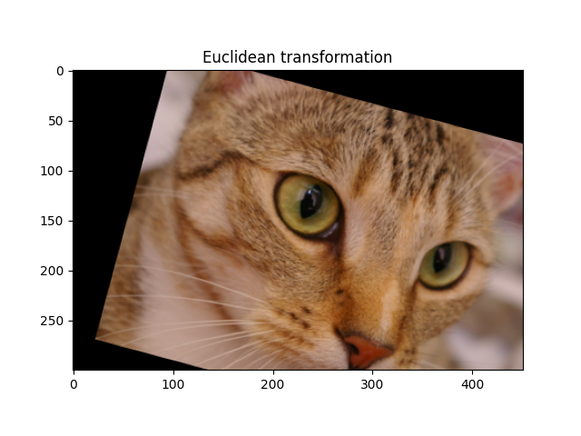
A Euclidean transformation, also called rigid transformation, preserves the Euclidean distance between pairs of points. It can be described as a rotation about the origin followed by a translation.

tform = transform.EuclideanTransform(rotation=np.pi / 12.0, translation=(100, -20))
print(tform.params)

[[  0.96592583  -0.25881905 100.        ]
 [  0.25881905   0.96592583 -20.        ]
 [  0.           0.           1.        ]]

Now let’s apply this transformation to an image. Because we are trying to reconstruct the image after transformation, it is not useful to see where a coordinate from the input image ends up in the output, which is what the transform gives us. Instead, for every pixel (coordinate) in the output image, we want to figure out where in the input image it comes from. Therefore, we need to use the inverse of tform, rather than tform directly.

img = img_as_float(data.chelsea())
tf_img = transform.warp(img, tform.inverse)
fig, ax = plt.subplots()
ax.imshow(tf_img)
_ = ax.set_title('Euclidean transformation')

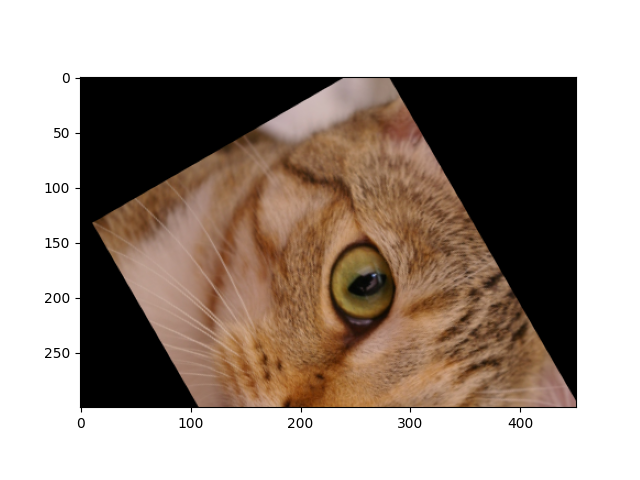
For a rotation around the center of the image, one can compose a translation to change the origin, a rotation, and finally the inverse of the first translation.

rotation = transform.EuclideanTransform(rotation=np.pi / 3)
shift = transform.EuclideanTransform(translation=-np.array(img.shape[:2]) / 2)
# Compose transforms by multiplying their matrices
matrix = np.linalg.inv(shift.params) @ rotation.params @ shift.params
tform = transform.EuclideanTransform(matrix)
tf_img = transform.warp(img, tform.inverse)
fig, ax = plt.subplots()
_ = ax.imshow(tf_img)

Similarity transformation

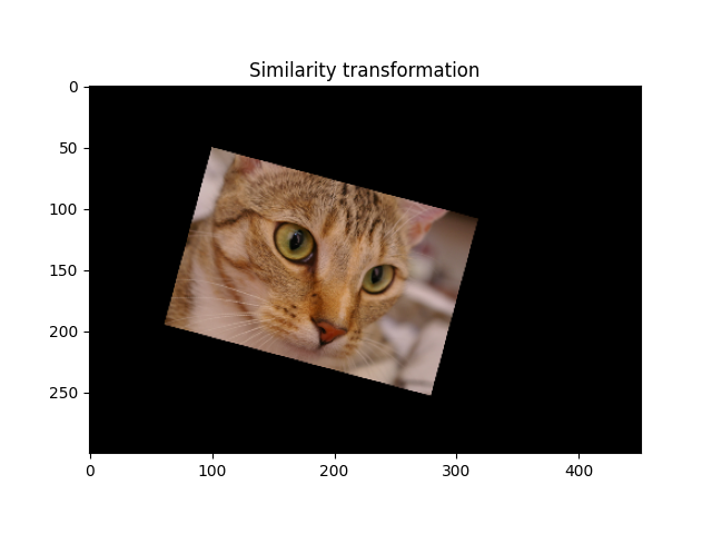
A similarity transformation preserves the shape of objects. It combines scaling, translation and rotation.

tform = transform.SimilarityTransform(
    scale=0.5, rotation=np.pi / 12, translation=(100, 50)
)
print(tform.params)
tf_img = transform.warp(img, tform.inverse)
fig, ax = plt.subplots()
ax.imshow(tf_img)
_ = ax.set_title('Similarity transformation')

[[  0.48296291  -0.12940952 100.        ]
 [  0.12940952   0.48296291  50.        ]
 [  0.           0.           1.        ]]

Affine transformation

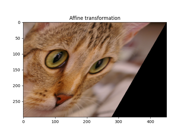
An affine transformation preserves lines (hence the alignment of objects), as well as parallelism between lines. It can be decomposed into a similarity transform and a shear transformation.

tform = transform.AffineTransform(
    shear=np.pi / 6,
)
print(tform.params)
tf_img = transform.warp(img, tform.inverse)
fig, ax = plt.subplots()
ax.imshow(tf_img)
_ = ax.set_title('Affine transformation')

[[ 1.         -0.57735027  0.        ]
 [ 0.          1.          0.        ]
 [ 0.          0.          1.        ]]

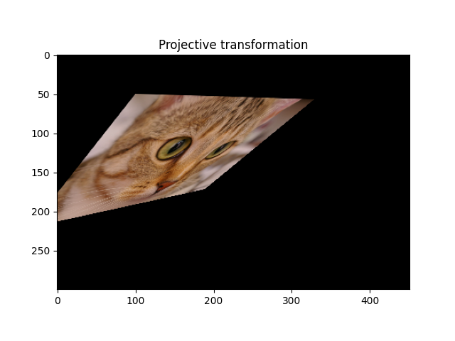
Projective transformation (homographies)

A homography, also called projective transformation, preserves lines but not necessarily parallelism.

matrix = np.array([[1, -0.5, 100], [0.1, 0.9, 50], [0.0015, 0.0015, 1]])
tform = transform.ProjectiveTransform(matrix=matrix)
tf_img = transform.warp(img, tform.inverse)
fig, ax = plt.subplots()
ax.imshow(tf_img)
ax.set_title('Projective transformation')

plt.show()

See also

• Using geometric transformations for composing transformations or estimating their parameters

• Rescale, resize, and downscale for simple rescaling and resizing operations

• skimage.transform.rotate() for rotating an image around its center