skimage.morphology#
Morphological algorithms, e.g., closing, opening, skeletonization.
Perform an area closing of the image. |
|
Perform an area opening of the image. |
|
Generates a ball-shaped footprint. |
|
Return black top hat of an image. |
|
Return grayscale morphological closing of an image. |
|
Compute the convex hull image of a binary image. |
|
Compute the convex hull image of individual objects in a binary image. |
|
Perform a diameter closing of the image. |
|
Perform a diameter opening of the image. |
|
Generates a flat, diamond-shaped footprint. |
|
Return grayscale morphological dilation of an image. |
|
Generates a flat, disk-shaped footprint. |
|
Generates a flat, ellipse-shaped footprint. |
|
Return grayscale morphological erosion of an image. |
|
Mask corresponding to a flood fill. |
|
Perform flood filling on an image. |
|
Convert a footprint sequence into an equivalent ndarray. |
|
Generate a rectangular or hyper-rectangular footprint. |
|
Determine all maxima of the image with height >= h. |
|
Determine all minima of the image with depth >= h. |
|
Return binary morphological closing of an image. |
|
Return binary morphological dilation of an image. |
|
Return binary morphological erosion of an image. |
|
Return binary morphological opening of an image. |
|
Label connected regions of an integer array. |
|
Find local maxima of n-dimensional array. |
|
Find local minima of n-dimensional array. |
|
Build the max tree from an image. |
|
Determine all local maxima of the image. |
|
Compute the medial axis transform of a binary image. |
|
Mirror each dimension in the footprint. |
|
Generates an octagon shaped footprint. |
|
Generates a octahedron-shaped footprint. |
|
Return grayscale morphological opening of an image. |
|
Pad the footprint to an odd size along each dimension. |
|
Perform a morphological reconstruction of an image. |
|
Remove objects, in specified order, until remaining are a minimum distance apart. |
|
Remove contiguous holes smaller than the specified size. |
|
Remove objects smaller than the specified size. |
|
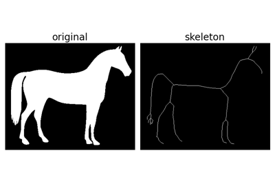
Compute the skeleton of the input image via thinning. |
|
Generates a star shaped footprint. |
|
Perform morphological thinning of a binary image. |
|
Return white top hat of an image. |
- skimage.morphology.area_closing(image, area_threshold=64, connectivity=1, parent=None, tree_traverser=None)[source]#
Perform an area closing of the image.
Area closing removes all dark structures of an image with a surface smaller than area_threshold. The output image is larger than or equal to the input image for every pixel and all local minima have at least a surface of area_threshold pixels.
Area closings are similar to morphological closings, but they do not use a fixed footprint, but rather a deformable one, with surface = area_threshold.
In the binary case, area closings are equivalent to remove_small_holes; this operator is thus extended to gray-level images.
Technically, this operator is based on the max-tree representation of the image.
- Parameters:
- imagendarray
The input image for which the area_closing is to be calculated. This image can be of any type.
- area_thresholdunsigned int
The size parameter (number of pixels). The default value is arbitrarily chosen to be 64.
- connectivityunsigned int, optional
The neighborhood connectivity. The integer represents the maximum number of orthogonal steps to reach a neighbor. In 2D, it is 1 for a 4-neighborhood and 2 for a 8-neighborhood. Default value is 1.
- parentndarray, int64, optional
Parent image representing the max tree of the inverted image. The value of each pixel is the index of its parent in the ravelled array. See Note for further details.
- tree_traverser1D array, int64, optional
The ordered pixel indices (referring to the ravelled array). The pixels are ordered such that every pixel is preceded by its parent (except for the root which has no parent).
- Returns:
- outputndarray
Output image of the same shape and type as input image.
See also
Notes
If a max-tree representation (parent and tree_traverser) are given to the function, they must be calculated from the inverted image for this function, i.e.: >>> P, S = max_tree(invert(f)) >>> closed = diameter_closing(f, 3, parent=P, tree_traverser=S)
References
[1]Vincent L., Proc. “Grayscale area openings and closings, their efficient implementation and applications”, EURASIP Workshop on Mathematical Morphology and its Applications to Signal Processing, Barcelona, Spain, pp.22-27, May 1993.
[2]Soille, P., “Morphological Image Analysis: Principles and Applications” (Chapter 6), 2nd edition (2003), ISBN 3540429883. DOI:10.1007/978-3-662-05088-0
[3]Salembier, P., Oliveras, A., & Garrido, L. (1998). Antiextensive Connected Operators for Image and Sequence Processing. IEEE Transactions on Image Processing, 7(4), 555-570. DOI:10.1109/83.663500
[4]Najman, L., & Couprie, M. (2006). Building the component tree in quasi-linear time. IEEE Transactions on Image Processing, 15(11), 3531-3539. DOI:10.1109/TIP.2006.877518
[5]Carlinet, E., & Geraud, T. (2014). A Comparative Review of Component Tree Computation Algorithms. IEEE Transactions on Image Processing, 23(9), 3885-3895. DOI:10.1109/TIP.2014.2336551
Examples
We create an image (quadratic function with a minimum in the center and 4 additional local minima.
>>> w = 12
>>> x, y = np.mgrid[0:w,0:w]
>>> f = 180 + 0.2*((x - w/2)**2 + (y-w/2)**2)
>>> f[2:3,1:5] = 160; f[2:4,9:11] = 140; f[9:11,2:4] = 120
>>> f[9:10,9:11] = 100; f[10,10] = 100
>>> f = f.astype(int)
We can calculate the area closing:
>>> closed = area_closing(f, 8, connectivity=1)
All small minima are removed, and the remaining minima have at least a size of 8.
- skimage.morphology.area_opening(image, area_threshold=64, connectivity=1, parent=None, tree_traverser=None)[source]#
Perform an area opening of the image.
Area opening removes all bright structures of an image with a surface smaller than area_threshold. The output image is thus the largest image smaller than the input for which all local maxima have at least a surface of area_threshold pixels.
Area openings are similar to morphological openings, but they do not use a fixed footprint, but rather a deformable one, with surface = area_threshold. Consequently, the area_opening with area_threshold=1 is the identity.
In the binary case, area openings are equivalent to remove_small_objects; this operator is thus extended to gray-level images.
Technically, this operator is based on the max-tree representation of the image.
- Parameters:
- imagendarray
The input image for which the area_opening is to be calculated. This image can be of any type.
- area_thresholdunsigned int
The size parameter (number of pixels). The default value is arbitrarily chosen to be 64.
- connectivityunsigned int, optional
The neighborhood connectivity. The integer represents the maximum number of orthogonal steps to reach a neighbor. In 2D, it is 1 for a 4-neighborhood and 2 for a 8-neighborhood. Default value is 1.
- parentndarray, int64, optional
Parent image representing the max tree of the image. The value of each pixel is the index of its parent in the ravelled array.
- tree_traverser1D array, int64, optional
The ordered pixel indices (referring to the ravelled array). The pixels are ordered such that every pixel is preceded by its parent (except for the root which has no parent).
- Returns:
- outputndarray
Output image of the same shape and type as the input image.
See also
References
[1]Vincent L., Proc. “Grayscale area openings and closings, their efficient implementation and applications”, EURASIP Workshop on Mathematical Morphology and its Applications to Signal Processing, Barcelona, Spain, pp.22-27, May 1993.
[2]Soille, P., “Morphological Image Analysis: Principles and Applications” (Chapter 6), 2nd edition (2003), ISBN 3540429883. DOI:10.1007/978-3-662-05088-0
[3]Salembier, P., Oliveras, A., & Garrido, L. (1998). Antiextensive Connected Operators for Image and Sequence Processing. IEEE Transactions on Image Processing, 7(4), 555-570. DOI:10.1109/83.663500
[4]Najman, L., & Couprie, M. (2006). Building the component tree in quasi-linear time. IEEE Transactions on Image Processing, 15(11), 3531-3539. DOI:10.1109/TIP.2006.877518
[5]Carlinet, E., & Geraud, T. (2014). A Comparative Review of Component Tree Computation Algorithms. IEEE Transactions on Image Processing, 23(9), 3885-3895. DOI:10.1109/TIP.2014.2336551
Examples
We create an image (quadratic function with a maximum in the center and 4 additional local maxima.
>>> w = 12
>>> x, y = np.mgrid[0:w,0:w]
>>> f = 20 - 0.2*((x - w/2)**2 + (y-w/2)**2)
>>> f[2:3,1:5] = 40; f[2:4,9:11] = 60; f[9:11,2:4] = 80
>>> f[9:10,9:11] = 100; f[10,10] = 100
>>> f = f.astype(int)
We can calculate the area opening:
>>> open = area_opening(f, 8, connectivity=1)
The peaks with a surface smaller than 8 are removed.
- skimage.morphology.ball(radius, dtype=<class 'numpy.uint8'>, *, strict_radius=True, decomposition=None)[source]#
Generates a ball-shaped footprint.
This is the 3D equivalent of a disk. A pixel is within the neighborhood if the Euclidean distance between it and the origin is no greater than radius.
- Parameters:
- radiusfloat
The radius of the ball-shaped footprint.
- Returns:
- footprintndarray or tuple
The footprint where elements of the neighborhood are 1 and 0 otherwise.
- Other Parameters:
- dtypedata-type, optional
The data type of the footprint.
- strict_radiusbool, optional
If False, extend the radius by 0.5. This allows the circle to expand further within a cube that remains of size
2 * radius + 1along each axis. This parameter is ignored if decomposition is not None.- decomposition{None, ‘sequence’}, optional
If None, a single array is returned. For ‘sequence’, a tuple of smaller footprints is returned. Applying this series of smaller footprints will given a result equivalent to a single, larger footprint, but with better computational performance. For ball footprints, the sequence decomposition is not exactly equivalent to decomposition=None. See Notes for more details.
Notes
The disk produced by the decomposition=’sequence’ mode is not identical to that with decomposition=None. Here we extend the approach taken in [1] for disks to the 3D case, using 3-dimensional extensions of the “square”, “diamond” and “t-shaped” elements from that publication. All of these elementary elements have size
(3,) * ndim. We numerically computed the number of repetitions of each element that gives the closest match to the ball computed with kwargsstrict_radius=False, decomposition=None.Empirically, the equivalent composite footprint to the sequence decomposition approaches a rhombicuboctahedron (26-faces [2]).
References
[1]Park, H and Chin R.T. Decomposition of structuring elements for optimal implementation of morphological operations. In Proceedings: 1997 IEEE Workshop on Nonlinear Signal and Image Processing, London, UK. https://www.iwaenc.org/proceedings/1997/nsip97/pdf/scan/ns970226.pdf
- skimage.morphology.black_tophat(image, footprint=None, out=None, *, mode='reflect', cval=0.0)[source]#
Return black top hat of an image.
The black top hat of an image is defined as its morphological closing minus the original image. This operation returns the dark spots of the image that are smaller than the footprint. Note that dark spots in the original image are bright spots after the black top hat.
- Parameters:
- imagendarray
Image array.
- footprintndarray or tuple, optional
The neighborhood expressed as a 2-D array of 1’s and 0’s. If None, use a cross-shaped footprint (connectivity=1). The footprint can also be provided as a sequence of smaller footprints as described in the notes below.
- outndarray, optional
The array to store the result of the morphology. If None is passed, a new array will be allocated.
- modestr, optional
The
modeparameter determines how the array borders are handled. Valid modes are: ‘reflect’, ‘constant’, ‘nearest’, ‘mirror’, ‘wrap’, ‘max’, ‘min’, or ‘ignore’. Seeskimage.morphology.closing(). Default is ‘reflect’.- cvalscalar, optional
Value to fill past edges of input if
modeis ‘constant’. Default is 0.0.Added in version 0.23:
modeandcvalwere added in 0.23.
- Returns:
- outarray, same shape and type as
image The result of the morphological black top hat.
- outarray, same shape and type as
See also
Notes
The footprint can also be a provided as a sequence of 2-tuples where the first element of each 2-tuple is a footprint ndarray and the second element is an integer describing the number of times it should be iterated. For example
footprint=[(np.ones((9, 1)), 1), (np.ones((1, 9)), 1)]would apply a 9x1 footprint followed by a 1x9 footprint resulting in a net effect that is the same asfootprint=np.ones((9, 9)), but with lower computational cost. Most of the builtin footprints such asskimage.morphology.disk()provide an option to automatically generate a footprint sequence of this type.References
Examples
>>> # Change dark peak to bright peak and subtract background
>>> import numpy as np
>>> from skimage.morphology import footprint_rectangle
>>> dark_on_gray = np.array([[7, 6, 6, 6, 7],
...                          [6, 5, 4, 5, 6],
...                          [6, 4, 0, 4, 6],
...                          [6, 5, 4, 5, 6],
...                          [7, 6, 6, 6, 7]], dtype=np.uint8)
>>> black_tophat(dark_on_gray, footprint_rectangle((3, 3)))
array([[0, 0, 0, 0, 0],
       [0, 0, 1, 0, 0],
       [0, 1, 5, 1, 0],
       [0, 0, 1, 0, 0],
       [0, 0, 0, 0, 0]], dtype=uint8)
- skimage.morphology.closing(image, footprint=None, out=None, *, mode='reflect', cval=0.0)[source]#
Return grayscale morphological closing of an image.
The morphological closing of an image is defined as a dilation followed by an erosion. Closing can remove small dark spots (i.e. “pepper”) and connect small bright cracks. This tends to “close” up (dark) gaps between (bright) features.
- Parameters:
- imagendarray
Image array.
- footprintndarray or tuple, optional
The neighborhood expressed as a 2-D array of 1’s and 0’s. If None, use a cross-shaped footprint (connectivity=1). The footprint can also be provided as a sequence of smaller footprints as described in the notes below.
- outndarray, optional
The array to store the result of the morphology. If None, a new array will be allocated.
- modestr, optional
The
modeparameter determines how the array borders are handled. Valid modes are: ‘reflect’, ‘constant’, ‘nearest’, ‘mirror’, ‘wrap’, ‘max’, ‘min’, or ‘ignore’. If ‘ignore’, pixels outside the image domain are assumed to be the maximum for the image’s dtype in the erosion, and minimum in the dilation, which causes them to not influence the result. Default is ‘reflect’.- cvalscalar, optional
Value to fill past edges of input if
modeis ‘constant’. Default is 0.0.Added in version 0.23:
modeandcvalwere added in 0.23.
- Returns:
- closingarray, same shape and type as
image The result of the morphological closing.
- closingarray, same shape and type as
Notes
The footprint can also be a provided as a sequence of 2-tuples where the first element of each 2-tuple is a footprint ndarray and the second element is an integer describing the number of times it should be iterated. For example
footprint=[(np.ones((9, 1)), 1), (np.ones((1, 9)), 1)]would apply a 9x1 footprint followed by a 1x9 footprint resulting in a net effect that is the same asfootprint=np.ones((9, 9)), but with lower computational cost. Most of the builtin footprints such asskimage.morphology.disk()provide an option to automatically generate a footprint sequence of this type.Examples
>>> # Close a gap between two bright lines
>>> import numpy as np
>>> from skimage.morphology import footprint_rectangle
>>> broken_line = np.array([[0, 0, 0, 0, 0],
...                         [0, 0, 0, 0, 0],
...                         [1, 1, 0, 1, 1],
...                         [0, 0, 0, 0, 0],
...                         [0, 0, 0, 0, 0]], dtype=np.uint8)
>>> closing(broken_line, footprint_rectangle((3, 3)))
array([[0, 0, 0, 0, 0],
       [0, 0, 0, 0, 0],
       [1, 1, 1, 1, 1],
       [0, 0, 0, 0, 0],
       [0, 0, 0, 0, 0]], dtype=uint8)
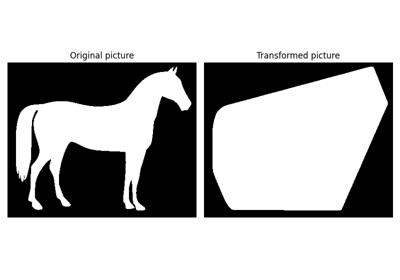
- skimage.morphology.convex_hull_image(image, offset_coordinates=True, tolerance=1e-10, include_borders=True)[source]#
Compute the convex hull image of a binary image.
The convex hull is the set of pixels included in the smallest convex polygon that surround all white pixels in the input image.
- Parameters:
- imagearray
Binary input image. This array is cast to bool before processing.
- offset_coordinatesbool, optional
If
True, a pixel at coordinate, e.g., (4, 7) will be represented by coordinates (3.5, 7), (4.5, 7), (4, 6.5), and (4, 7.5). This adds some “extent” to a pixel when computing the hull.- tolerancefloat, optional
Tolerance when determining whether a point is inside the hull. Due to numerical floating point errors, a tolerance of 0 can result in some points erroneously being classified as being outside the hull.
- include_bordersbool, optional
If
False, vertices/edges are excluded from the final hull mask.
- Returns:
- hull(M, N) array of bool
Binary image with pixels in convex hull set to True.
References
- skimage.morphology.convex_hull_object(image, *, connectivity=2)[source]#
Compute the convex hull image of individual objects in a binary image.
The convex hull is the set of pixels included in the smallest convex polygon that surround all white pixels in the input image.
- Parameters:
- image(M, N) ndarray
Binary input image.
- connectivity{1, 2}, int, optional
Determines the neighbors of each pixel. Adjacent elements within a squared distance of
connectivityfrom pixel center are considered neighbors.:1-connectivity 2-connectivity [ ] [ ] [ ] [ ] | \ | / [ ]--[x]--[ ] [ ]--[x]--[ ] | / | \ [ ] [ ] [ ] [ ]
- Returns:
- hullndarray of bool
Binary image with pixels inside convex hull set to
True.
Notes
This function uses
skimage.morphology.labelto define unique objects, finds the convex hull of each usingconvex_hull_image, and combines these regions with logical OR. Be aware the convex hulls of unconnected objects may overlap in the result. If this is suspected, consider using convex_hull_image separately on each object or adjustconnectivity.
- skimage.morphology.diameter_closing(image, diameter_threshold=8, connectivity=1, parent=None, tree_traverser=None)[source]#
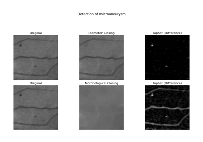
Perform a diameter closing of the image.
Diameter closing removes all dark structures of an image with maximal extension smaller than diameter_threshold. The maximal extension is defined as the maximal extension of the bounding box. The operator is also called Bounding Box Closing. In practice, the result is similar to a morphological closing, but long and thin structures are not removed.
Technically, this operator is based on the max-tree representation of the image.
- Parameters:
- imagendarray
The input image for which the diameter_closing is to be calculated. This image can be of any type.
- diameter_thresholdunsigned int
The maximal extension parameter (number of pixels). The default value is 8.
- connectivityunsigned int, optional
The neighborhood connectivity. The integer represents the maximum number of orthogonal steps to reach a neighbor. In 2D, it is 1 for a 4-neighborhood and 2 for a 8-neighborhood. Default value is 1.
- parentndarray, int64, optional
Precomputed parent image representing the max tree of the inverted image. This function is fast, if precomputed parent and tree_traverser are provided. See Note for further details.
- tree_traverser1D array, int64, optional
Precomputed traverser, where the pixels are ordered such that every pixel is preceded by its parent (except for the root which has no parent). This function is fast, if precomputed parent and tree_traverser are provided. See Note for further details.
- Returns:
- outputndarray
Output image of the same shape and type as input image.
See also
Notes
If a max-tree representation (parent and tree_traverser) are given to the function, they must be calculated from the inverted image for this function, i.e.: >>> P, S = max_tree(invert(f)) >>> closed = diameter_closing(f, 3, parent=P, tree_traverser=S)
References
[1]Walter, T., & Klein, J.-C. (2002). Automatic Detection of Microaneurysms in Color Fundus Images of the Human Retina by Means of the Bounding Box Closing. In A. Colosimo, P. Sirabella, A. Giuliani (Eds.), Medical Data Analysis. Lecture Notes in Computer Science, vol 2526, pp. 210-220. Springer Berlin Heidelberg. DOI:10.1007/3-540-36104-9_23
[2]Carlinet, E., & Geraud, T. (2014). A Comparative Review of Component Tree Computation Algorithms. IEEE Transactions on Image Processing, 23(9), 3885-3895. DOI:10.1109/TIP.2014.2336551
Examples
We create an image (quadratic function with a minimum in the center and 4 additional local minima.
>>> w = 12
>>> x, y = np.mgrid[0:w,0:w]
>>> f = 180 + 0.2*((x - w/2)**2 + (y-w/2)**2)
>>> f[2:3,1:5] = 160; f[2:4,9:11] = 140; f[9:11,2:4] = 120
>>> f[9:10,9:11] = 100; f[10,10] = 100
>>> f = f.astype(int)
We can calculate the diameter closing:
>>> closed = diameter_closing(f, 3, connectivity=1)
All small minima with a maximal extension of 2 or less are removed. The remaining minima have all a maximal extension of at least 3.
- skimage.morphology.diameter_opening(image, diameter_threshold=8, connectivity=1, parent=None, tree_traverser=None)[source]#
Perform a diameter opening of the image.
Diameter opening removes all bright structures of an image with maximal extension smaller than diameter_threshold. The maximal extension is defined as the maximal extension of the bounding box. The operator is also called Bounding Box Opening. In practice, the result is similar to a morphological opening, but long and thin structures are not removed.
Technically, this operator is based on the max-tree representation of the image.
- Parameters:
- imagendarray
The input image for which the area_opening is to be calculated. This image can be of any type.
- diameter_thresholdunsigned int
The maximal extension parameter (number of pixels). The default value is 8.
- connectivityunsigned int, optional
The neighborhood connectivity. The integer represents the maximum number of orthogonal steps to reach a neighbor. In 2D, it is 1 for a 4-neighborhood and 2 for a 8-neighborhood. Default value is 1.
- parentndarray, int64, optional
Parent image representing the max tree of the image. The value of each pixel is the index of its parent in the ravelled array.
- tree_traverser1D array, int64, optional
The ordered pixel indices (referring to the ravelled array). The pixels are ordered such that every pixel is preceded by its parent (except for the root which has no parent).
- Returns:
- outputndarray
Output image of the same shape and type as the input image.
See also
References
[1]Walter, T., & Klein, J.-C. (2002). Automatic Detection of Microaneurysms in Color Fundus Images of the Human Retina by Means of the Bounding Box Closing. In A. Colosimo, P. Sirabella, A. Giuliani (Eds.), Medical Data Analysis. Lecture Notes in Computer Science, vol 2526, pp. 210-220. Springer Berlin Heidelberg. DOI:10.1007/3-540-36104-9_23
[2]Carlinet, E., & Geraud, T. (2014). A Comparative Review of Component Tree Computation Algorithms. IEEE Transactions on Image Processing, 23(9), 3885-3895. DOI:10.1109/TIP.2014.2336551
Examples
We create an image (quadratic function with a maximum in the center and 4 additional local maxima.
>>> w = 12
>>> x, y = np.mgrid[0:w,0:w]
>>> f = 20 - 0.2*((x - w/2)**2 + (y-w/2)**2)
>>> f[2:3,1:5] = 40; f[2:4,9:11] = 60; f[9:11,2:4] = 80
>>> f[9:10,9:11] = 100; f[10,10] = 100
>>> f = f.astype(int)
We can calculate the diameter opening:
>>> open = diameter_opening(f, 3, connectivity=1)
The peaks with a maximal extension of 2 or less are removed. The remaining peaks have all a maximal extension of at least 3.
- skimage.morphology.diamond(radius, dtype=<class 'numpy.uint8'>, *, decomposition=None)[source]#
Generates a flat, diamond-shaped footprint.
A pixel is part of the neighborhood (i.e. labeled 1) if the city block/Manhattan distance between it and the center of the neighborhood is no greater than radius.
- Parameters:
- radiusint
The radius of the diamond-shaped footprint.
- Returns:
- footprintndarray or tuple
The footprint where elements of the neighborhood are 1 and 0 otherwise. When
decompositionis None, this is just a numpy.ndarray. Otherwise, this will be a tuple whose length is equal to the number of unique structuring elements to apply (see Notes for more detail)
- Other Parameters:
- dtypedata-type, optional
The data type of the footprint.
- decomposition{None, ‘sequence’}, optional
If None, a single array is returned. For ‘sequence’, a tuple of smaller footprints is returned. Applying this series of smaller footprints will given an identical result to a single, larger footprint, but with better computational performance. See Notes for more details.
Notes
When
decompositionis not None, each element of thefootprinttuple is a 2-tuple of the form(ndarray, num_iter)that specifies a footprint array and the number of iterations it is to be applied.For either binary or grayscale morphology, using
decomposition='sequence'was observed to have a performance benefit, with the magnitude of the benefit increasing with increasing footprint size.
- skimage.morphology.dilation(image, footprint=None, out=None, *, mode='reflect', cval=0.0)[source]#
Return grayscale morphological dilation of an image.
Morphological dilation sets the value of a pixel to the maximum over all pixel values within a local neighborhood centered about it. The values where the footprint is 1 define this neighborhood. Dilation enlarges bright regions and shrinks dark regions.
- Parameters:
- imagendarray
Image array.
- footprintndarray or tuple, optional
The neighborhood expressed as a 2-D array of 1’s and 0’s. If None, use a cross-shaped footprint (connectivity=1). The footprint can also be provided as a sequence of smaller footprints as described in the notes below.
- outndarray, optional
The array to store the result of the morphology. If None is passed, a new array will be allocated.
- modestr, optional
The
modeparameter determines how the array borders are handled. Valid modes are: ‘reflect’, ‘constant’, ‘nearest’, ‘mirror’, ‘wrap’, ‘max’, ‘min’, or ‘ignore’. If ‘min’ or ‘ignore’, pixels outside the image domain are assumed to be the maximum for the image’s dtype, which causes them to not influence the result. Default is ‘reflect’.- cvalscalar, optional
Value to fill past edges of input if
modeis ‘constant’. Default is 0.0.Added in version 0.23:
modeandcvalwere added in 0.23.
- Returns:
- dilateduint8 array, same shape and type as
image The result of the morphological dilation.
- dilateduint8 array, same shape and type as
Notes
For
uint8(anduint16up to a certain bit-depth) data, the lower algorithm complexity makes theskimage.filters.rank.maximum()function more efficient for larger images and footprints.The footprint can also be a provided as a sequence of 2-tuples where the first element of each 2-tuple is a footprint ndarray and the second element is an integer describing the number of times it should be iterated. For example
footprint=[(np.ones((9, 1)), 1), (np.ones((1, 9)), 1)]would apply a 9x1 footprint followed by a 1x9 footprint resulting in a net effect that is the same asfootprint=np.ones((9, 9)), but with lower computational cost. Most of the builtin footprints such asskimage.morphology.disk()provide an option to automatically generate a footprint sequence of this type.For non-symmetric footprints,
skimage.morphology.binary_dilation()andskimage.morphology.dilation()produce an output that differs:binary_dilationmirrors the footprint, whereasdilationdoes not.skimage.morphology.mirror_footprint()is available to correct for this.Examples
>>> # Dilation enlarges bright regions
>>> import numpy as np
>>> from skimage.morphology import footprint_rectangle
>>> bright_pixel = np.array([[0, 0, 0, 0, 0],
...                          [0, 0, 0, 0, 0],
...                          [0, 0, 1, 0, 0],
...                          [0, 0, 0, 0, 0],
...                          [0, 0, 0, 0, 0]], dtype=np.uint8)
>>> dilation(bright_pixel, footprint_rectangle((3, 3)))
array([[0, 0, 0, 0, 0],
       [0, 1, 1, 1, 0],
       [0, 1, 1, 1, 0],
       [0, 1, 1, 1, 0],
       [0, 0, 0, 0, 0]], dtype=uint8)
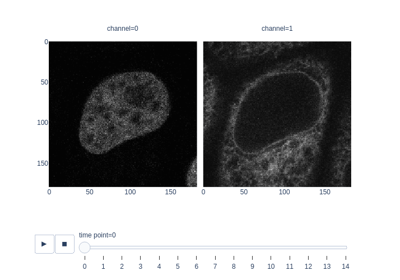
Measure fluorescence intensity at the nuclear envelope
Measure fluorescence intensity at the nuclear envelope
- skimage.morphology.disk(radius, dtype=<class 'numpy.uint8'>, *, strict_radius=True, decomposition=None)[source]#
Generates a flat, disk-shaped footprint.
A pixel is within the neighborhood if the Euclidean distance between it and the origin is no greater than radius (This is only approximately True, when
decomposition == 'sequence').- Parameters:
- radiusint
The radius of the disk-shaped footprint.
- Returns:
- footprintndarray
The footprint where elements of the neighborhood are 1 and 0 otherwise.
- Other Parameters:
- dtypedata-type, optional
The data type of the footprint.
- strict_radiusbool, optional
If False, extend the radius by 0.5. This allows the circle to expand further within a cube that remains of size
2 * radius + 1along each axis. This parameter is ignored if decomposition is not None.- decomposition{None, ‘sequence’, ‘crosses’}, optional
If None, a single array is returned. For ‘sequence’, a tuple of smaller footprints is returned. Applying this series of smaller footprints will given a result equivalent to a single, larger footprint, but with better computational performance. For disk footprints, the ‘sequence’ or ‘crosses’ decompositions are not always exactly equivalent to
decomposition=None. See Notes for more details.
Notes
When
decompositionis not None, each element of thefootprinttuple is a 2-tuple of the form(ndarray, num_iter)that specifies a footprint array and the number of iterations it is to be applied.The disk produced by the
decomposition='sequence'mode may not be identical to that withdecomposition=None. A disk footprint can be approximated by applying a series of smaller footprints of extent 3 along each axis. Specific solutions for this are given in [1] for the case of 2D disks with radius 2 through 10. Here, we numerically computed the number of repetitions of each element that gives the closest match to the disk computed with kwargsstrict_radius=False, decomposition=None.Empirically, the series decomposition at large radius approaches a hexadecagon (a 16-sided polygon [2]). In [3], the authors demonstrate that a hexadecagon is the closest approximation to a disk that can be achieved for decomposition with footprints of shape (3, 3).
The disk produced by the
decomposition='crosses'is often but not always identical to that withdecomposition=None. It tends to give a closer approximation thandecomposition='sequence', at a performance that is fairly comparable. The individual cross-shaped elements are not limited to extent (3, 3) in size. Unlike the ‘seqeuence’ decomposition, the ‘crosses’ decomposition can also accurately approximate the shape of disks withstrict_radius=True. The method is based on an adaption of algorithm 1 given in [4].References
[1]Park, H and Chin R.T. Decomposition of structuring elements for optimal implementation of morphological operations. In Proceedings: 1997 IEEE Workshop on Nonlinear Signal and Image Processing, London, UK. https://www.iwaenc.org/proceedings/1997/nsip97/pdf/scan/ns970226.pdf
[3]Vanrell, M and Vitrià, J. Optimal 3 × 3 decomposable disks for morphological transformations. Image and Vision Computing, Vol. 15, Issue 11, 1997. DOI:10.1016/S0262-8856(97)00026-7
[4]Li, D. and Ritter, G.X. Decomposition of Separable and Symmetric Convex Templates. Proc. SPIE 1350, Image Algebra and Morphological Image Processing, (1 November 1990). DOI:10.1117/12.23608
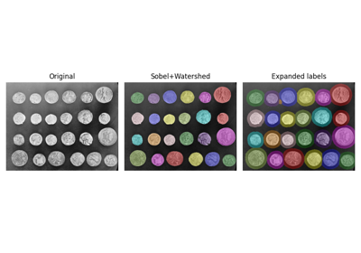
Removing small objects in grayscale images with a top hat filter
Removing small objects in grayscale images with a top hat filter
- skimage.morphology.ellipse(width, height, dtype=<class 'numpy.uint8'>, *, decomposition=None)[source]#
Generates a flat, ellipse-shaped footprint.
Every pixel along the perimeter of ellipse satisfies the equation
(x/width+1)**2 + (y/height+1)**2 = 1.- Parameters:
- widthint
The width of the ellipse-shaped footprint.
- heightint
The height of the ellipse-shaped footprint.
- Returns:
- footprintndarray
The footprint where elements of the neighborhood are 1 and 0 otherwise. The footprint will have shape
(2 * height + 1, 2 * width + 1).
- Other Parameters:
- dtypedata-type, optional
The data type of the footprint.
- decomposition{None, ‘crosses’}, optional
If None, a single array is returned. For ‘sequence’, a tuple of smaller footprints is returned. Applying this series of smaller footprints will given an identical result to a single, larger footprint, but with better computational performance. See Notes for more details.
Notes
When
decompositionis not None, each element of thefootprinttuple is a 2-tuple of the form(ndarray, num_iter)that specifies a footprint array and the number of iterations it is to be applied.The ellipse produced by the
decomposition='crosses'is often but not always identical to that withdecomposition=None. The method is based on an adaption of algorithm 1 given in [1].References
[1]Li, D. and Ritter, G.X. Decomposition of Separable and Symmetric Convex Templates. Proc. SPIE 1350, Image Algebra and Morphological Image Processing, (1 November 1990). DOI:10.1117/12.23608
Examples
>>> from skimage.morphology import footprints
>>> footprints.ellipse(5, 3)
array([[0, 0, 1, 1, 1, 1, 1, 1, 1, 0, 0],
       [1, 1, 1, 1, 1, 1, 1, 1, 1, 1, 1],
       [1, 1, 1, 1, 1, 1, 1, 1, 1, 1, 1],
       [1, 1, 1, 1, 1, 1, 1, 1, 1, 1, 1],
       [1, 1, 1, 1, 1, 1, 1, 1, 1, 1, 1],
       [1, 1, 1, 1, 1, 1, 1, 1, 1, 1, 1],
       [0, 0, 1, 1, 1, 1, 1, 1, 1, 0, 0]], dtype=uint8)
- skimage.morphology.erosion(image, footprint=None, out=None, *, mode='reflect', cval=0.0)[source]#
Return grayscale morphological erosion of an image.
Morphological erosion sets a pixel at (i,j) to the minimum over all pixels in the neighborhood centered at (i,j). Erosion shrinks bright regions and enlarges dark regions.
- Parameters:
- imagendarray
Image array.
- footprintndarray or tuple, optional
The neighborhood expressed as a 2-D array of 1’s and 0’s. If None, use a cross-shaped footprint (connectivity=1). The footprint can also be provided as a sequence of smaller footprints as described in the notes below.
- outndarrays, optional
The array to store the result of the morphology. If None is passed, a new array will be allocated.
- modestr, optional
The
modeparameter determines how the array borders are handled. Valid modes are: ‘reflect’, ‘constant’, ‘nearest’, ‘mirror’, ‘wrap’, ‘max’, ‘min’, or ‘ignore’. If ‘max’ or ‘ignore’, pixels outside the image domain are assumed to be the maximum for the image’s dtype, which causes them to not influence the result. Default is ‘reflect’.- cvalscalar, optional
Value to fill past edges of input if
modeis ‘constant’. Default is 0.0.Added in version 0.23:
modeandcvalwere added in 0.23.
- Returns:
- erodedarray, same shape as
image The result of the morphological erosion.
- erodedarray, same shape as
Notes
For
uint8(anduint16up to a certain bit-depth) data, the lower algorithm complexity makes theskimage.filters.rank.minimum()function more efficient for larger images and footprints.The footprint can also be a provided as a sequence of 2-tuples where the first element of each 2-tuple is a footprint ndarray and the second element is an integer describing the number of times it should be iterated. For example
footprint=[(np.ones((9, 1)), 1), (np.ones((1, 9)), 1)]would apply a 9x1 footprint followed by a 1x9 footprint resulting in a net effect that is the same asfootprint=np.ones((9, 9)), but with lower computational cost. Most of the builtin footprints such asskimage.morphology.disk()provide an option to automatically generate a footprint sequence of this type.For even-sized footprints,
skimage.morphology.binary_erosion()and this function produce an output that differs: one is shifted by one pixel compared to the other.skimage.morphology.pad_footprint()is available to account for this.Examples
>>> # Erosion shrinks bright regions
>>> import numpy as np
>>> from skimage.morphology import footprint_rectangle
>>> bright_square = np.array([[0, 0, 0, 0, 0],
...                           [0, 1, 1, 1, 0],
...                           [0, 1, 1, 1, 0],
...                           [0, 1, 1, 1, 0],
...                           [0, 0, 0, 0, 0]], dtype=np.uint8)
>>> erosion(bright_square, footprint_rectangle((3, 3)))
array([[0, 0, 0, 0, 0],
       [0, 0, 0, 0, 0],
       [0, 0, 1, 0, 0],
       [0, 0, 0, 0, 0],
       [0, 0, 0, 0, 0]], dtype=uint8)
Measure fluorescence intensity at the nuclear envelope
Measure fluorescence intensity at the nuclear envelope
- skimage.morphology.flood(image, seed_point, *, footprint=None, connectivity=None, tolerance=None)[source]#
Mask corresponding to a flood fill.
Starting at a specific
seed_point, connected points equal or withintoleranceof the seed value are found.- Parameters:
- imagendarray
An n-dimensional array.
- seed_pointtuple or int
The point in
imageused as the starting point for the flood fill. If the image is 1D, this point may be given as an integer.- footprintndarray, optional
The footprint (structuring element) used to determine the neighborhood of each evaluated pixel. It must contain only 1’s and 0’s, have the same number of dimensions as
image. If not given, all adjacent pixels are considered as part of the neighborhood (fully connected).- connectivityint, optional
A number used to determine the neighborhood of each evaluated pixel. Adjacent pixels whose squared distance from the center is less than or equal to
connectivityare considered neighbors. Ignored iffootprintis not None.- tolerancefloat or int, optional
If None (default), adjacent values must be strictly equal to the initial value of
imageatseed_point. This is fastest. If a value is given, a comparison will be done at every point and if within tolerance of the initial value will also be filled (inclusive).
- Returns:
- maskndarray
A Boolean array with the same shape as
imageis returned, with True values for areas connected to and equal (or within tolerance of) the seed point. All other values are False.
Notes
The conceptual analogy of this operation is the ‘paint bucket’ tool in many raster graphics programs. This function returns just the mask representing the fill.
If indices are desired rather than masks for memory reasons, the user can simply run
numpy.nonzeroon the result, save the indices, and discard this mask.Examples
>>> from skimage.morphology import flood
>>> image = np.zeros((4, 7), dtype=int)
>>> image[1:3, 1:3] = 1
>>> image[3, 0] = 1
>>> image[1:3, 4:6] = 2
>>> image[3, 6] = 3
>>> image
array([[0, 0, 0, 0, 0, 0, 0],
       [0, 1, 1, 0, 2, 2, 0],
       [0, 1, 1, 0, 2, 2, 0],
       [1, 0, 0, 0, 0, 0, 3]])
Fill connected ones with 5, with full connectivity (diagonals included):
>>> mask = flood(image, (1, 1))
>>> image_flooded = image.copy()
>>> image_flooded[mask] = 5
>>> image_flooded
array([[0, 0, 0, 0, 0, 0, 0],
       [0, 5, 5, 0, 2, 2, 0],
       [0, 5, 5, 0, 2, 2, 0],
       [5, 0, 0, 0, 0, 0, 3]])
Fill connected ones with 5, excluding diagonal points (connectivity 1):
>>> mask = flood(image, (1, 1), connectivity=1)
>>> image_flooded = image.copy()
>>> image_flooded[mask] = 5
>>> image_flooded
array([[0, 0, 0, 0, 0, 0, 0],
       [0, 5, 5, 0, 2, 2, 0],
       [0, 5, 5, 0, 2, 2, 0],
       [1, 0, 0, 0, 0, 0, 3]])
Fill with a tolerance:
>>> mask = flood(image, (0, 0), tolerance=1)
>>> image_flooded = image.copy()
>>> image_flooded[mask] = 5
>>> image_flooded
array([[5, 5, 5, 5, 5, 5, 5],
       [5, 5, 5, 5, 2, 2, 5],
       [5, 5, 5, 5, 2, 2, 5],
       [5, 5, 5, 5, 5, 5, 3]])
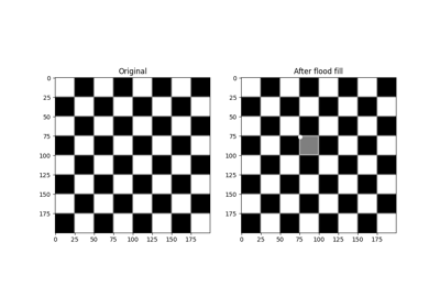
- skimage.morphology.flood_fill(image, seed_point, new_value, *, footprint=None, connectivity=None, tolerance=None, in_place=False)[source]#
Perform flood filling on an image.
Starting at a specific
seed_point, connected points equal or withintoleranceof the seed value are found, then set tonew_value.- Parameters:
- imagendarray
An n-dimensional array.
- seed_pointtuple or int
The point in
imageused as the starting point for the flood fill. If the image is 1D, this point may be given as an integer.- new_value
imagetype New value to set the entire fill. This must be chosen in agreement with the dtype of
image.- footprintndarray, optional
The footprint (structuring element) used to determine the neighborhood of each evaluated pixel. It must contain only 1’s and 0’s, have the same number of dimensions as
image. If not given, all adjacent pixels are considered as part of the neighborhood (fully connected).- connectivityint, optional
A number used to determine the neighborhood of each evaluated pixel. Adjacent pixels whose squared distance from the center is less than or equal to
connectivityare considered neighbors. Ignored iffootprintis not None.- tolerancefloat or int, optional
If None (default), adjacent values must be strictly equal to the value of
imageatseed_pointto be filled. This is fastest. If a tolerance is provided, adjacent points with values within plus or minus tolerance from the seed point are filled (inclusive).- in_placebool, optional
If True, flood filling is applied to
imagein place. If False, the flood filled result is returned without modifying the inputimage(default).
- Returns:
- filledndarray
An array with the same shape as
imageis returned, with values in areas connected to and equal (or within tolerance of) the seed point replaced withnew_value.
Notes
The conceptual analogy of this operation is the ‘paint bucket’ tool in many raster graphics programs.
Examples
>>> from skimage.morphology import flood_fill
>>> image = np.zeros((4, 7), dtype=int)
>>> image[1:3, 1:3] = 1
>>> image[3, 0] = 1
>>> image[1:3, 4:6] = 2
>>> image[3, 6] = 3
>>> image
array([[0, 0, 0, 0, 0, 0, 0],
       [0, 1, 1, 0, 2, 2, 0],
       [0, 1, 1, 0, 2, 2, 0],
       [1, 0, 0, 0, 0, 0, 3]])
Fill connected ones with 5, with full connectivity (diagonals included):
>>> flood_fill(image, (1, 1), 5)
array([[0, 0, 0, 0, 0, 0, 0],
       [0, 5, 5, 0, 2, 2, 0],
       [0, 5, 5, 0, 2, 2, 0],
       [5, 0, 0, 0, 0, 0, 3]])
Fill connected ones with 5, excluding diagonal points (connectivity 1):
>>> flood_fill(image, (1, 1), 5, connectivity=1)
array([[0, 0, 0, 0, 0, 0, 0],
       [0, 5, 5, 0, 2, 2, 0],
       [0, 5, 5, 0, 2, 2, 0],
       [1, 0, 0, 0, 0, 0, 3]])
Fill with a tolerance:
>>> flood_fill(image, (0, 0), 5, tolerance=1)
array([[5, 5, 5, 5, 5, 5, 5],
       [5, 5, 5, 5, 2, 2, 5],
       [5, 5, 5, 5, 2, 2, 5],
       [5, 5, 5, 5, 5, 5, 3]])
- skimage.morphology.footprint_from_sequence(footprints)[source]#
Convert a footprint sequence into an equivalent ndarray.
- Parameters:
- footprintstuple of 2-tuples
A sequence of footprint tuples where the first element of each tuple is an array corresponding to a footprint and the second element is the number of times it is to be applied. Currently, all footprints should have odd size.
- Returns:
- footprintndarray
An single array equivalent to applying the sequence of
footprints.
- skimage.morphology.footprint_rectangle(shape, *, dtype=<class 'numpy.uint8'>, decomposition=None)[source]#
Generate a rectangular or hyper-rectangular footprint.
Generates, depending on the length and dimensions requested with
shape, a square, rectangle, cube, cuboid, or even higher-dimensional versions of these shapes.- Parameters:
- shapetuple[int, …]
The length of the footprint in each dimension. The length of the sequence determines the number of dimensions of the footprint.
- dtypedata-type, optional
The data type of the footprint.
- decomposition{None, ‘separable’, ‘sequence’}, optional
If None, a single array is returned. For ‘sequence’, a tuple of smaller footprints is returned. Applying this series of smaller footprints will give an identical result to a single, larger footprint, but often with better computational performance. See Notes for more details. With ‘separable’, this function uses separable 1D footprints for each axis. Whether ‘sequence’ or ‘separable’ is computationally faster may be architecture-dependent.
- Returns:
- footprintarray or tuple[tuple[ndarray, int], …]
A footprint consisting only of ones, i.e. every pixel belongs to the neighborhood. When
decompositionis None, this is just an array. Otherwise, this will be a tuple whose length is equal to the number of unique structuring elements to apply (see Examples for more detail).
Examples
>>> import skimage as ski
>>> ski.morphology.footprint_rectangle((3, 5))
array([[1, 1, 1, 1, 1],
       [1, 1, 1, 1, 1],
       [1, 1, 1, 1, 1]], dtype=uint8)
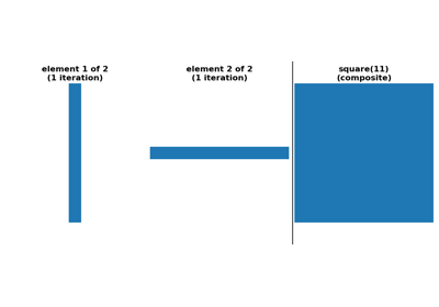
Decomposition will return multiple footprints that combine into a simple footprint of the requested shape.
>>> ski.morphology.footprint_rectangle((9, 9), decomposition="sequence")
((array([[1, 1, 1],
         [1, 1, 1],
         [1, 1, 1]], dtype=uint8),
  4),)
"sequence"makes sure that the decomposition only returns 1D footprints.>>> ski.morphology.footprint_rectangle((3, 5), decomposition="separable") ((array([[1], [1], [1]], dtype=uint8), 1), (array([[1, 1, 1, 1, 1]], dtype=uint8), 1))
Generate a 5-dimensional hypercube with 3 samples in each dimension
>>> ski.morphology.footprint_rectangle((3,) * 5).shape
(3, 3, 3, 3, 3)
- skimage.morphology.h_maxima(image, h, footprint=None)[source]#
Determine all maxima of the image with height >= h.
The local maxima are defined as connected sets of pixels with equal gray level strictly greater than the gray level of all pixels in direct neighborhood of the set.
A local maximum M of height h is a local maximum for which there is at least one path joining M with an equal or higher local maximum on which the minimal value is f(M) - h (i.e. the values along the path are not decreasing by more than h with respect to the maximum’s value) and no path to an equal or higher local maximum for which the minimal value is greater.
The global maxima of the image are also found by this function.
- Parameters:
- imagendarray
The input image for which the maxima are to be calculated.
- hunsigned integer
The minimal height of all extracted maxima.
- footprintndarray, optional
The neighborhood expressed as an n-D array of 1’s and 0’s. Default is the ball of radius 1 according to the maximum norm (i.e. a 3x3 square for 2D images, a 3x3x3 cube for 3D images, etc.)
- Returns:
- h_maxndarray
The local maxima of height >= h and the global maxima. The resulting image is a binary image, where pixels belonging to the determined maxima take value 1, the others take value 0.
See also
References
[1]Soille, P., “Morphological Image Analysis: Principles and Applications” (Chapter 6), 2nd edition (2003), ISBN 3540429883.
Examples
>>> import numpy as np
>>> from skimage.morphology import extrema
We create an image (quadratic function with a maximum in the center and 4 additional constant maxima. The heights of the maxima are: 1, 21, 41, 61, 81
>>> w = 10
>>> x, y = np.mgrid[0:w,0:w]
>>> f = 20 - 0.2*((x - w/2)**2 + (y-w/2)**2)
>>> f[2:4,2:4] = 40; f[2:4,7:9] = 60; f[7:9,2:4] = 80; f[7:9,7:9] = 100
>>> f = f.astype(int)
We can calculate all maxima with a height of at least 40:
>>> maxima = extrema.h_maxima(f, 40)
The resulting image will contain 3 local maxima.
- skimage.morphology.h_minima(image, h, footprint=None)[source]#
Determine all minima of the image with depth >= h.
The local minima are defined as connected sets of pixels with equal gray level strictly smaller than the gray levels of all pixels in direct neighborhood of the set.
A local minimum M of depth h is a local minimum for which there is at least one path joining M with an equal or lower local minimum on which the maximal value is f(M) + h (i.e. the values along the path are not increasing by more than h with respect to the minimum’s value) and no path to an equal or lower local minimum for which the maximal value is smaller.
The global minima of the image are also found by this function.
- Parameters:
- imagendarray
The input image for which the minima are to be calculated.
- hunsigned integer
The minimal depth of all extracted minima.
- footprintndarray, optional
The neighborhood expressed as an n-D array of 1’s and 0’s. Default is the ball of radius 1 according to the maximum norm (i.e. a 3x3 square for 2D images, a 3x3x3 cube for 3D images, etc.)
- Returns:
- h_minndarray
The local minima of depth >= h and the global minima. The resulting image is a binary image, where pixels belonging to the determined minima take value 1, the others take value 0.
See also
References
[1]Soille, P., “Morphological Image Analysis: Principles and Applications” (Chapter 6), 2nd edition (2003), ISBN 3540429883.
Examples
>>> import numpy as np
>>> from skimage.morphology import extrema
We create an image (quadratic function with a minimum in the center and 4 additional constant maxima. The depth of the minima are: 1, 21, 41, 61, 81
>>> w = 10
>>> x, y = np.mgrid[0:w,0:w]
>>> f = 180 + 0.2*((x - w/2)**2 + (y-w/2)**2)
>>> f[2:4,2:4] = 160; f[2:4,7:9] = 140; f[7:9,2:4] = 120; f[7:9,7:9] = 100
>>> f = f.astype(int)
We can calculate all minima with a depth of at least 40:
>>> minima = extrema.h_minima(f, 40)
The resulting image will contain 3 local minima.
- skimage.morphology.isotropic_closing(image, radius, out=None, spacing=None)[source]#
Return binary morphological closing of an image.
Compared to the more general
skimage.morphology.closing(), this function only supports binary inputs and circular footprints. However, it performs typically faster for large (circular) footprints. This works by thresholding the exact Euclidean distance map [1], [2]. The implementation is based on: func:scipy.ndimage.distance_transform_edt.- Parameters:
- imagendarray
Binary input image.
- radiusfloat
The radius of the footprint used for the operation.
- outndarray of bool, optional
The array to store the result of the morphology. If None, is passed, a new array will be allocated.
- spacingfloat, or sequence of float, optional
Spacing of elements along each dimension. If a sequence, must be of length equal to the input’s dimension (number of axes). If a single number, this value is used for all axes. If not specified, a grid spacing of unity is implied.
- Returns:
- closedndarray of bool
The result of the morphological closing.
References
[1]Cuisenaire, O. and Macq, B., “Fast Euclidean morphological operators using local distance transformation by propagation, and applications,” Image Processing And Its Applications, 1999. Seventh International Conference on (Conf. Publ. No. 465), 1999, pp. 856-860 vol.2. DOI:10.1049/cp:19990446
[2]Ingemar Ragnemalm, Fast erosion and dilation by contour processing and thresholding of distance maps, Pattern Recognition Letters, Volume 13, Issue 3, 1992, Pages 161-166. DOI:10.1016/0167-8655(92)90055-5
Examples
Close gap between two bright lines
>>> import numpy as np
>>> import skimage as ski
>>> image = np.array([[0, 0, 0, 0, 0],
...                   [0, 0, 0, 0, 0],
...                   [1, 1, 0, 1, 1],
...                   [0, 0, 0, 0, 0],
...                   [0, 0, 0, 0, 0]], dtype=bool)
>>> result = ski.morphology.isotropic_closing(image, radius=1)
>>> result.view(np.uint8)
array([[0, 0, 0, 0, 0],
       [0, 0, 0, 0, 0],
       [1, 1, 0, 1, 1],
       [0, 0, 0, 0, 0],
       [0, 0, 0, 0, 0]], dtype=uint8)
- skimage.morphology.isotropic_dilation(image, radius, out=None, spacing=None)[source]#
Return binary morphological dilation of an image.
Compared to the more general
skimage.morphology.dilation(), this function only supports binary inputs and circular footprints. However, it performs typically faster for large (circular) footprints. This works by applying a threshold to the exact Euclidean distance map of the inverted image [1], [2]. The implementation is based on: func:scipy.ndimage.distance_transform_edt.- Parameters:
- imagendarray
Binary input image.
- radiusfloat
The radius of the footprint used for the operation.
- outndarray of bool, optional
The array to store the result of the morphology. If None is passed, a new array will be allocated.
- spacingfloat, or sequence of float, optional
Spacing of elements along each dimension. If a sequence, must be of length equal to the input’s dimension (number of axes). If a single number, this value is used for all axes. If not specified, a grid spacing of unity is implied.
- Returns:
- dilatedndarray of bool
The result of the morphological dilation with values in
[False, True].
References
[1]Cuisenaire, O. and Macq, B., “Fast Euclidean morphological operators using local distance transformation by propagation, and applications,” Image Processing And Its Applications, 1999. Seventh International Conference on (Conf. Publ. No. 465), 1999, pp. 856-860 vol.2. DOI:10.1049/cp:19990446
[2]Ingemar Ragnemalm, Fast erosion and dilation by contour processing and thresholding of distance maps, Pattern Recognition Letters, Volume 13, Issue 3, 1992, Pages 161-166. DOI:10.1016/0167-8655(92)90055-5
Examples
Dilation enlarges bright regions
>>> import numpy as np
>>> import skimage as ski
>>> image = np.array([[0, 0, 0, 0, 0],
...                   [0, 0, 0, 0, 0],
...                   [0, 0, 1, 0, 0],
...                   [0, 0, 1, 1, 0],
...                   [0, 0, 0, 0, 0]], dtype=bool)
>>> result = ski.morphology.isotropic_dilation(image, radius=1)
>>> result.view(np.uint8)
array([[0, 0, 0, 0, 0],
       [0, 0, 1, 0, 0],
       [0, 1, 1, 1, 0],
       [0, 1, 1, 1, 1],
       [0, 0, 1, 1, 0]], dtype=uint8)
- skimage.morphology.isotropic_erosion(image, radius, out=None, spacing=None)[source]#
Return binary morphological erosion of an image.
Compared to the more general
skimage.morphology.erosion(), this function only supports binary inputs and circular footprints. However, it performs typically faster for large (circular) footprints. This works by applying a threshold to the exact Euclidean distance map of the image [1], [2]. The implementation is based on: func:scipy.ndimage.distance_transform_edt.- Parameters:
- imagendarray
Binary input image.
- radiusfloat
The radius of the footprint used for the operation.
- outndarray of bool, optional
The array to store the result of the morphology. If None, a new array will be allocated.
- spacingfloat, or sequence of float, optional
Spacing of elements along each dimension. If a sequence, must be of length equal to the input’s dimension (number of axes). If a single number, this value is used for all axes. If not specified, a grid spacing of unity is implied.
- Returns:
- erodedndarray of bool
The result of the morphological erosion taking values in
[False, True].
References
[1]Cuisenaire, O. and Macq, B., “Fast Euclidean morphological operators using local distance transformation by propagation, and applications,” Image Processing And Its Applications, 1999. Seventh International Conference on (Conf. Publ. No. 465), 1999, pp. 856-860 vol.2. DOI:10.1049/cp:19990446
[2]Ingemar Ragnemalm, Fast erosion and dilation by contour processing and thresholding of distance maps, Pattern Recognition Letters, Volume 13, Issue 3, 1992, Pages 161-166. DOI:10.1016/0167-8655(92)90055-5
Examples
Erosion shrinks bright regions
>>> import numpy as np
>>> import skimage as ski
>>> image = np.array([[0, 0, 1, 0, 0],
...                   [0, 1, 1, 1, 0],
...                   [0, 1, 1, 1, 0],
...                   [0, 1, 1, 1, 0],
...                   [0, 0, 0, 0, 0]], dtype=bool)
>>> result = ski.morphology.isotropic_erosion(image, radius=1)
>>> result.view(np.uint8)
array([[0, 0, 0, 0, 0],
       [0, 0, 1, 0, 0],
       [0, 0, 1, 0, 0],
       [0, 0, 0, 0, 0],
       [0, 0, 0, 0, 0]], dtype=uint8)
- skimage.morphology.isotropic_opening(image, radius, out=None, spacing=None)[source]#
Return binary morphological opening of an image.
Compared to the more general
skimage.morphology.opening(), this function only supports binary inputs and circular footprints. However, it performs typically faster for large (circular) footprints. This works by thresholding the exact Euclidean distance map [1], [2]. The implementation is based on: func:scipy.ndimage.distance_transform_edt.- Parameters:
- imagendarray
Binary input image.
- radiusfloat
The radius of the footprint used for the operation.
- outndarray of bool, optional
The array to store the result of the morphology. If None is passed, a new array will be allocated.
- spacingfloat, or sequence of float, optional
Spacing of elements along each dimension. If a sequence, must be of length equal to the input’s dimension (number of axes). If a single number, this value is used for all axes. If not specified, a grid spacing of unity is implied.
- Returns:
- openedndarray of bool
The result of the morphological opening.
References
[1]Cuisenaire, O. and Macq, B., “Fast Euclidean morphological operators using local distance transformation by propagation, and applications,” Image Processing And Its Applications, 1999. Seventh International Conference on (Conf. Publ. No. 465), 1999, pp. 856-860 vol.2. DOI:10.1049/cp:19990446
[2]Ingemar Ragnemalm, Fast erosion and dilation by contour processing and thresholding of distance maps, Pattern Recognition Letters, Volume 13, Issue 3, 1992, Pages 161-166. DOI:10.1016/0167-8655(92)90055-5
Examples
Remove connection between two bright regions
>>> import numpy as np
>>> import skimage as ski
>>> image = np.array([[1, 0, 0, 0, 1],
...                   [1, 1, 0, 1, 1],
...                   [1, 1, 1, 1, 1],
...                   [1, 1, 0, 1, 1],
...                   [1, 0, 0, 0, 1]], dtype=bool)
>>> result = ski.morphology.isotropic_opening(image, radius=1)
>>> result.view(np.uint8)
array([[1, 0, 0, 0, 1],
       [1, 1, 0, 1, 1],
       [1, 1, 1, 1, 1],
       [1, 1, 0, 1, 1],
       [1, 0, 0, 0, 1]], dtype=uint8)
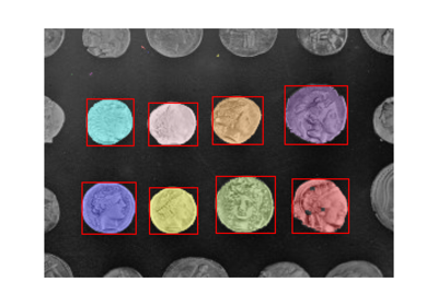
- skimage.morphology.label(label_image, background=None, return_num=False, connectivity=None)[source]#
Label connected regions of an integer array.
Two pixels are connected when they are neighbors and have the same value. In 2D, they can be neighbors either in a 1- or 2-connected sense. The value refers to the maximum number of orthogonal hops to consider a pixel/voxel a neighbor:
1-connectivity     2-connectivity     diagonal connection close-up

     [ ]           [ ]  [ ]  [ ]             [ ]
      |               \  |  /                 |  <- hop 2
[ ]--[x]--[ ]      [ ]--[x]--[ ]        [x]--[ ]
      |               /  |  \             hop 1
     [ ]           [ ]  [ ]  [ ]
- Parameters:
- label_imagendarray of dtype int
Image to label.
- backgroundint, optional
Consider all pixels with this value as background pixels, and label them as 0. By default, 0-valued pixels are considered as background pixels.
- return_numbool, optional
Whether to return the number of assigned labels.
- connectivityint, optional
Maximum number of orthogonal hops to consider a pixel/voxel as a neighbor. Accepted values are ranging from 1 to input.ndim. If
None, a full connectivity ofinput.ndimis used.
- Returns:
- labelsndarray of dtype int
Labeled array, where all connected regions are assigned the same integer value.
- numint, optional
Number of labels, which equals the maximum label index and is only returned if return_num is
True.
References
[1]Christophe Fiorio and Jens Gustedt, “Two linear time Union-Find strategies for image processing”, Theoretical Computer Science 154 (1996), pp. 165-181.
[2]Kensheng Wu, Ekow Otoo and Arie Shoshani, “Optimizing connected component labeling algorithms”, Paper LBNL-56864, 2005, Lawrence Berkeley National Laboratory (University of California), http://repositories.cdlib.org/lbnl/LBNL-56864
Examples
>>> import numpy as np
>>> x = np.eye(3).astype(int)
>>> print(x)
[[1 0 0]
 [0 1 0]
 [0 0 1]]
>>> print(label(x, connectivity=1))
[[1 0 0]
 [0 2 0]
 [0 0 3]]
>>> print(label(x, connectivity=2))
[[1 0 0]
 [0 1 0]
 [0 0 1]]
>>> print(label(x, background=-1))
[[1 2 2]
 [2 1 2]
 [2 2 1]]
>>> x = np.array([[1, 0, 0],
...               [1, 1, 5],
...               [0, 0, 0]])
>>> print(label(x))
[[1 0 0]
 [1 1 2]
 [0 0 0]]
- skimage.morphology.local_maxima(image, footprint=None, connectivity=None, indices=False, allow_borders=True)[source]#
Find local maxima of n-dimensional array.
The local maxima are defined as connected sets of pixels with equal gray level (plateaus) strictly greater than the gray levels of all pixels in the neighborhood.
- Parameters:
- imagendarray
An n-dimensional array.
- footprintndarray, optional
The footprint (structuring element) used to determine the neighborhood of each evaluated pixel (
Truedenotes a connected pixel). It must be a boolean array and have the same number of dimensions asimage. If neitherfootprintnorconnectivityare given, all adjacent pixels are considered as part of the neighborhood.- connectivityint, optional
A number used to determine the neighborhood of each evaluated pixel. Adjacent pixels whose squared distance from the center is less than or equal to
connectivityare considered neighbors. Ignored iffootprintis not None.- indicesbool, optional
If True, the output will be a tuple of one-dimensional arrays representing the indices of local maxima in each dimension. If False, the output will be a boolean array with the same shape as
image.- allow_bordersbool, optional
If true, plateaus that touch the image border are valid maxima.
- Returns:
- maximandarray or tuple[ndarray]
If
indicesis false, a boolean array with the same shape asimageis returned withTrueindicating the position of local maxima (Falseotherwise). Ifindicesis true, a tuple of one-dimensional arrays containing the coordinates (indices) of all found maxima.
- Warns:
- UserWarning
If
allow_bordersis false and any dimension of the givenimageis shorter than 3 samples, maxima can’t exist and a warning is shown.
Notes
This function operates on the following ideas:
Make a first pass over the image’s last dimension and flag candidates for local maxima by comparing pixels in only one direction. If the pixels aren’t connected in the last dimension all pixels are flagged as candidates instead.
For each candidate:
Perform a flood-fill to find all connected pixels that have the same gray value and are part of the plateau.
Consider the connected neighborhood of a plateau: if no bordering sample has a higher gray level, mark the plateau as a definite local maximum.
Examples
>>> from skimage.morphology import local_maxima
>>> image = np.zeros((4, 7), dtype=int)
>>> image[1:3, 1:3] = 1
>>> image[3, 0] = 1
>>> image[1:3, 4:6] = 2
>>> image[3, 6] = 3
>>> image
array([[0, 0, 0, 0, 0, 0, 0],
       [0, 1, 1, 0, 2, 2, 0],
       [0, 1, 1, 0, 2, 2, 0],
       [1, 0, 0, 0, 0, 0, 3]])
Find local maxima by comparing to all neighboring pixels (maximal connectivity):
>>> local_maxima(image)
array([[False, False, False, False, False, False, False],
       [False,  True,  True, False, False, False, False],
       [False,  True,  True, False, False, False, False],
       [ True, False, False, False, False, False,  True]])
>>> local_maxima(image, indices=True)
(array([1, 1, 2, 2, 3, 3]), array([1, 2, 1, 2, 0, 6]))
Find local maxima without comparing to diagonal pixels (connectivity 1):
>>> local_maxima(image, connectivity=1)
array([[False, False, False, False, False, False, False],
       [False,  True,  True, False,  True,  True, False],
       [False,  True,  True, False,  True,  True, False],
       [ True, False, False, False, False, False,  True]])
and exclude maxima that border the image edge:
>>> local_maxima(image, connectivity=1, allow_borders=False)
array([[False, False, False, False, False, False, False],
       [False,  True,  True, False,  True,  True, False],
       [False,  True,  True, False,  True,  True, False],
       [False, False, False, False, False, False, False]])
- skimage.morphology.local_minima(image, footprint=None, connectivity=None, indices=False, allow_borders=True)[source]#
Find local minima of n-dimensional array.
The local minima are defined as connected sets of pixels with equal gray level (plateaus) strictly smaller than the gray levels of all pixels in the neighborhood.
- Parameters:
- imagendarray
An n-dimensional array.
- footprintndarray, optional
The footprint (structuring element) used to determine the neighborhood of each evaluated pixel (
Truedenotes a connected pixel). It must be a boolean array and have the same number of dimensions asimage. If neitherfootprintnorconnectivityare given, all adjacent pixels are considered as part of the neighborhood.- connectivityint, optional
A number used to determine the neighborhood of each evaluated pixel. Adjacent pixels whose squared distance from the center is less than or equal to
connectivityare considered neighbors. Ignored iffootprintis not None.- indicesbool, optional
If True, the output will be a tuple of one-dimensional arrays representing the indices of local minima in each dimension. If False, the output will be a boolean array with the same shape as
image.- allow_bordersbool, optional
If true, plateaus that touch the image border are valid minima.
- Returns:
- minimandarray or tuple[ndarray]
If
indicesis false, a boolean array with the same shape asimageis returned withTrueindicating the position of local minima (Falseotherwise). Ifindicesis true, a tuple of one-dimensional arrays containing the coordinates (indices) of all found minima.
Notes
This function operates on the following ideas:
Make a first pass over the image’s last dimension and flag candidates for local minima by comparing pixels in only one direction. If the pixels aren’t connected in the last dimension all pixels are flagged as candidates instead.
For each candidate:
Perform a flood-fill to find all connected pixels that have the same gray value and are part of the plateau.
Consider the connected neighborhood of a plateau: if no bordering sample has a smaller gray level, mark the plateau as a definite local minimum.
Examples
>>> from skimage.morphology import local_minima
>>> image = np.zeros((4, 7), dtype=int)
>>> image[1:3, 1:3] = -1
>>> image[3, 0] = -1
>>> image[1:3, 4:6] = -2
>>> image[3, 6] = -3
>>> image
array([[ 0,  0,  0,  0,  0,  0,  0],
       [ 0, -1, -1,  0, -2, -2,  0],
       [ 0, -1, -1,  0, -2, -2,  0],
       [-1,  0,  0,  0,  0,  0, -3]])
Find local minima by comparing to all neighboring pixels (maximal connectivity):
>>> local_minima(image)
array([[False, False, False, False, False, False, False],
       [False,  True,  True, False, False, False, False],
       [False,  True,  True, False, False, False, False],
       [ True, False, False, False, False, False,  True]])
>>> local_minima(image, indices=True)
(array([1, 1, 2, 2, 3, 3]), array([1, 2, 1, 2, 0, 6]))
Find local minima without comparing to diagonal pixels (connectivity 1):
>>> local_minima(image, connectivity=1)
array([[False, False, False, False, False, False, False],
       [False,  True,  True, False,  True,  True, False],
       [False,  True,  True, False,  True,  True, False],
       [ True, False, False, False, False, False,  True]])
and exclude minima that border the image edge:
>>> local_minima(image, connectivity=1, allow_borders=False)
array([[False, False, False, False, False, False, False],
       [False,  True,  True, False,  True,  True, False],
       [False,  True,  True, False,  True,  True, False],
       [False, False, False, False, False, False, False]])
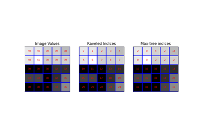
- skimage.morphology.max_tree(image, connectivity=1)[source]#
Build the max tree from an image.
Component trees represent the hierarchical structure of the connected components resulting from sequential thresholding operations applied to an image. A connected component at one level is parent of a component at a higher level if the latter is included in the first. A max-tree is an efficient representation of a component tree. A connected component at one level is represented by one reference pixel at this level, which is parent to all other pixels at that level and to the reference pixel at the level above. The max-tree is the basis for many morphological operators, namely connected operators.
- Parameters:
- imagendarray
The input image for which the max-tree is to be calculated. This image can be of any type.
- connectivityunsigned int, optional
The neighborhood connectivity. The integer represents the maximum number of orthogonal steps to reach a neighbor. In 2D, it is 1 for a 4-neighborhood and 2 for a 8-neighborhood. Default value is 1.
- Returns:
- parentndarray, int64
Array of same shape as image. The value of each pixel is the index of its parent in the ravelled array.
- tree_traverser1D array, int64
The ordered pixel indices (referring to the ravelled array). The pixels are ordered such that every pixel is preceded by its parent (except for the root which has no parent).
References
[1]Salembier, P., Oliveras, A., & Garrido, L. (1998). Antiextensive Connected Operators for Image and Sequence Processing. IEEE Transactions on Image Processing, 7(4), 555-570. DOI:10.1109/83.663500
[2]Berger, C., Geraud, T., Levillain, R., Widynski, N., Baillard, A., Bertin, E. (2007). Effective Component Tree Computation with Application to Pattern Recognition in Astronomical Imaging. In International Conference on Image Processing (ICIP) (pp. 41-44). DOI:10.1109/ICIP.2007.4379949
[3]Najman, L., & Couprie, M. (2006). Building the component tree in quasi-linear time. IEEE Transactions on Image Processing, 15(11), 3531-3539. DOI:10.1109/TIP.2006.877518
[4]Carlinet, E., & Geraud, T. (2014). A Comparative Review of Component Tree Computation Algorithms. IEEE Transactions on Image Processing, 23(9), 3885-3895. DOI:10.1109/TIP.2014.2336551
Examples
We create a small sample image (Figure 1 from [4]) and build the max-tree.
>>> image = np.array([[15, 13, 16], [12, 12, 10], [16, 12, 14]])
>>> P, S = max_tree(image, connectivity=2)
- skimage.morphology.max_tree_local_maxima(image, connectivity=1, parent=None, tree_traverser=None)[source]#
Determine all local maxima of the image.
The local maxima are defined as connected sets of pixels with equal gray level strictly greater than the gray levels of all pixels in direct neighborhood of the set. The function labels the local maxima.
Technically, the implementation is based on the max-tree representation of an image. The function is very efficient if the max-tree representation has already been computed. Otherwise, it is preferable to use the function local_maxima.
- Parameters:
- imagendarray
The input image for which the maxima are to be calculated.
- connectivityunsigned int, optional
The neighborhood connectivity. The integer represents the maximum number of orthogonal steps to reach a neighbor. In 2D, it is 1 for a 4-neighborhood and 2 for a 8-neighborhood. Default value is 1.
- parentndarray, int64, optional
The value of each pixel is the index of its parent in the ravelled array.
- tree_traverser1D array, int64, optional
The ordered pixel indices (referring to the ravelled array). The pixels are ordered such that every pixel is preceded by its parent (except for the root which has no parent).
- Returns:
- local_maxndarray, uint64
Labeled local maxima of the image.
References
[1]Vincent L., Proc. “Grayscale area openings and closings, their efficient implementation and applications”, EURASIP Workshop on Mathematical Morphology and its Applications to Signal Processing, Barcelona, Spain, pp.22-27, May 1993.
[2]Soille, P., “Morphological Image Analysis: Principles and Applications” (Chapter 6), 2nd edition (2003), ISBN 3540429883. DOI:10.1007/978-3-662-05088-0
[3]Salembier, P., Oliveras, A., & Garrido, L. (1998). Antiextensive Connected Operators for Image and Sequence Processing. IEEE Transactions on Image Processing, 7(4), 555-570. DOI:10.1109/83.663500
[4]Najman, L., & Couprie, M. (2006). Building the component tree in quasi-linear time. IEEE Transactions on Image Processing, 15(11), 3531-3539. DOI:10.1109/TIP.2006.877518
[5]Carlinet, E., & Geraud, T. (2014). A Comparative Review of Component Tree Computation Algorithms. IEEE Transactions on Image Processing, 23(9), 3885-3895. DOI:10.1109/TIP.2014.2336551
Examples
We create an image (quadratic function with a maximum in the center and 4 additional constant maxima.
>>> w = 10
>>> x, y = np.mgrid[0:w,0:w]
>>> f = 20 - 0.2*((x - w/2)**2 + (y-w/2)**2)
>>> f[2:4,2:4] = 40; f[2:4,7:9] = 60; f[7:9,2:4] = 80; f[7:9,7:9] = 100
>>> f = f.astype(int)
We can calculate all local maxima:
>>> maxima = max_tree_local_maxima(f)
The resulting image contains the labeled local maxima.
- skimage.morphology.medial_axis(image, mask=None, return_distance=False, *, rng=None)[source]#
Compute the medial axis transform of a binary image.
- Parameters:
- imagebinary ndarray, shape (M, N)
The image of the shape to skeletonize. If this input isn’t already a binary image, it gets converted into one: In this case, zero values are considered background (False), nonzero values are considered foreground (True).
- maskbinary ndarray, shape (M, N), optional
If a mask is given, only those elements in
imagewith a true value inmaskare used for computing the medial axis.- return_distancebool, optional
If true, the distance transform is returned as well as the skeleton.
- rng{
numpy.random.Generator, int}, optional Pseudo-random number generator. By default, a PCG64 generator is used (see
numpy.random.default_rng()). Ifrngis an int, it is used to seed the generator.The PRNG determines the order in which pixels are processed for tiebreaking.
Added in version 0.19.
- Returns:
- outndarray of bools
Medial axis transform of the image
- distndarray of ints, optional
Distance transform of the image (only returned if
return_distanceis True)
See also
Notes
This algorithm computes the medial axis transform of an image as the ridges of its distance transform.
- The different steps of the algorithm are as follows
A lookup table is used, that assigns 0 or 1 to each configuration of the 3x3 binary square, whether the central pixel should be removed or kept. We want a point to be removed if it has more than one neighbor and if removing it does not change the number of connected components.
The distance transform to the background is computed, as well as the cornerness of the pixel.
The foreground (value of 1) points are ordered by the distance transform, then the cornerness.
A cython function is called to reduce the image to its skeleton. It processes pixels in the order determined at the previous step, and removes or maintains a pixel according to the lookup table. Because of the ordering, it is possible to process all pixels in only one pass.
Examples
>>> square = np.zeros((7, 7), dtype=bool)
>>> square[1:-1, 2:-2] = 1
>>> square.view(np.uint8)
array([[0, 0, 0, 0, 0, 0, 0],
       [0, 0, 1, 1, 1, 0, 0],
       [0, 0, 1, 1, 1, 0, 0],
       [0, 0, 1, 1, 1, 0, 0],
       [0, 0, 1, 1, 1, 0, 0],
       [0, 0, 1, 1, 1, 0, 0],
       [0, 0, 0, 0, 0, 0, 0]], dtype=uint8)
>>> medial_axis(square).view(np.uint8)
array([[0, 0, 0, 0, 0, 0, 0],
       [0, 0, 1, 0, 1, 0, 0],
       [0, 0, 0, 1, 0, 0, 0],
       [0, 0, 0, 1, 0, 0, 0],
       [0, 0, 0, 1, 0, 0, 0],
       [0, 0, 1, 0, 1, 0, 0],
       [0, 0, 0, 0, 0, 0, 0]], dtype=uint8)
- skimage.morphology.mirror_footprint(footprint)[source]#
Mirror each dimension in the footprint.
- Parameters:
- footprintndarray or tuple
The input footprint or sequence of footprints
- Returns:
- invertedndarray or tuple
The footprint, mirrored along each dimension.
Examples
>>> footprint = np.array([[0, 0, 0],
...                       [0, 1, 1],
...                       [0, 1, 1]], np.uint8)
>>> mirror_footprint(footprint)
array([[1, 1, 0],
       [1, 1, 0],
       [0, 0, 0]], dtype=uint8)
- skimage.morphology.octagon(m, n, dtype=<class 'numpy.uint8'>, *, decomposition=None)[source]#
Generates an octagon shaped footprint.
For a given size of (m) horizontal and vertical sides and a given (n) height or width of slanted sides octagon is generated. The slanted sides are 45 or 135 degrees to the horizontal axis and hence the widths and heights are equal. The overall size of the footprint along a single axis will be
m + 2 * n.- Parameters:
- mint
The size of the horizontal and vertical sides.
- nint
The height or width of the slanted sides.
- Returns:
- footprintndarray or tuple
The footprint where elements of the neighborhood are 1 and 0 otherwise. When
decompositionis None, this is just a numpy.ndarray. Otherwise, this will be a tuple whose length is equal to the number of unique structuring elements to apply (see Notes for more detail)
- Other Parameters:
- dtypedata-type, optional
The data type of the footprint.
- decomposition{None, ‘sequence’}, optional
If None, a single array is returned. For ‘sequence’, a tuple of smaller footprints is returned. Applying this series of smaller footprints will given an identical result to a single, larger footprint, but with better computational performance. See Notes for more details.
Notes
When
decompositionis not None, each element of thefootprinttuple is a 2-tuple of the form(ndarray, num_iter)that specifies a footprint array and the number of iterations it is to be applied.For either binary or grayscale morphology, using
decomposition='sequence'was observed to have a performance benefit, with the magnitude of the benefit increasing with increasing footprint size.
- skimage.morphology.octahedron(radius, dtype=<class 'numpy.uint8'>, *, decomposition=None)[source]#
Generates a octahedron-shaped footprint.
This is the 3D equivalent of a diamond. A pixel is part of the neighborhood (i.e. labeled 1) if the city block/Manhattan distance between it and the center of the neighborhood is no greater than radius.
- Parameters:
- radiusint
The radius of the octahedron-shaped footprint.
- Returns:
- footprintndarray or tuple
The footprint where elements of the neighborhood are 1 and 0 otherwise. When
decompositionis None, this is just a numpy.ndarray. Otherwise, this will be a tuple whose length is equal to the number of unique structuring elements to apply (see Notes for more detail)
- Other Parameters:
- dtypedata-type, optional
The data type of the footprint.
- decomposition{None, ‘sequence’}, optional
If None, a single array is returned. For ‘sequence’, a tuple of smaller footprints is returned. Applying this series of smaller footprints will given an identical result to a single, larger footprint, but with better computational performance. See Notes for more details.
Notes
When
decompositionis not None, each element of thefootprinttuple is a 2-tuple of the form(ndarray, num_iter)that specifies a footprint array and the number of iterations it is to be applied.For either binary or grayscale morphology, using
decomposition='sequence'was observed to have a performance benefit, with the magnitude of the benefit increasing with increasing footprint size.
- skimage.morphology.opening(image, footprint=None, out=None, *, mode='reflect', cval=0.0)[source]#
Return grayscale morphological opening of an image.
The morphological opening of an image is defined as an erosion followed by a dilation. Opening can remove small bright spots (i.e. “salt”) and connect small dark cracks. This tends to “open” up (dark) gaps between (bright) features.
- Parameters:
- imagendarray
Image array.
- footprintndarray or tuple, optional
The neighborhood expressed as a 2-D array of 1’s and 0’s. If None, use a cross-shaped footprint (connectivity=1). The footprint can also be provided as a sequence of smaller footprints as described in the notes below.
- outndarray, optional
The array to store the result of the morphology. If None is passed, a new array will be allocated.
- modestr, optional
The
modeparameter determines how the array borders are handled. Valid modes are: ‘reflect’, ‘constant’, ‘nearest’, ‘mirror’, ‘wrap’, ‘max’, ‘min’, or ‘ignore’. If ‘ignore’, pixels outside the image domain are assumed to be the maximum for the image’s dtype in the erosion, and minimum in the dilation, which causes them to not influence the result. Default is ‘reflect’.- cvalscalar, optional
Value to fill past edges of input if
modeis ‘constant’. Default is 0.0.Added in version 0.23:
modeandcvalwere added in 0.23.
- Returns:
- openingarray, same shape and type as
image The result of the morphological opening.
- openingarray, same shape and type as
Notes
The footprint can also be a provided as a sequence of 2-tuples where the first element of each 2-tuple is a footprint ndarray and the second element is an integer describing the number of times it should be iterated. For example
footprint=[(np.ones((9, 1)), 1), (np.ones((1, 9)), 1)]would apply a 9x1 footprint followed by a 1x9 footprint resulting in a net effect that is the same asfootprint=np.ones((9, 9)), but with lower computational cost. Most of the builtin footprints such asskimage.morphology.disk()provide an option to automatically generate a footprint sequence of this type.Examples
>>> # Open up gap between two bright regions (but also shrink regions)
>>> import numpy as np
>>> from skimage.morphology import footprint_rectangle
>>> bad_connection = np.array([[1, 0, 0, 0, 1],
...                            [1, 1, 0, 1, 1],
...                            [1, 1, 1, 1, 1],
...                            [1, 1, 0, 1, 1],
...                            [1, 0, 0, 0, 1]], dtype=np.uint8)
>>> opening(bad_connection, footprint_rectangle((3, 3)))
array([[0, 0, 0, 0, 0],
       [1, 1, 0, 1, 1],
       [1, 1, 0, 1, 1],
       [1, 1, 0, 1, 1],
       [0, 0, 0, 0, 0]], dtype=uint8)
- skimage.morphology.pad_footprint(footprint, *, pad_end=True)[source]#
Pad the footprint to an odd size along each dimension.
- Parameters:
- footprintndarray or tuple
The input footprint or sequence of footprints
- pad_endbool, optional
If
True, pads at the end of each dimension (right side), otherwise pads on the front (left side).
- Returns:
- paddedndarray or tuple
The footprint, padded to an odd size along each dimension.
Examples
>>> footprint = np.array([[0, 0],
...                       [1, 1],
...                       [1, 1]], np.uint8)
>>> pad_footprint(footprint)
array([[0, 0, 0],
       [1, 1, 0],
       [1, 1, 0]], dtype=uint8)
- skimage.morphology.reconstruction(seed, mask, method='dilation', footprint=None, offset=None)[source]#
Perform a morphological reconstruction of an image.
Morphological reconstruction by dilation is similar to basic morphological dilation: high-intensity values will replace nearby low-intensity values. The basic dilation operator, however, uses a footprint to determine how far a value in the input image can spread. In contrast, reconstruction uses two images: a “seed” image, which specifies the values that spread, and a “mask” image, which gives the maximum allowed value at each pixel. The mask image, like the footprint, limits the spread of high-intensity values. Reconstruction by erosion is simply the inverse: low-intensity values spread from the seed image and are limited by the mask image, which represents the minimum allowed value.
Alternatively, you can think of reconstruction as a way to isolate the connected regions of an image. For dilation, reconstruction connects regions marked by local maxima in the seed image: neighboring pixels less-than-or-equal-to those seeds are connected to the seeded region. Local maxima with values larger than the seed image will get truncated to the seed value.
- Parameters:
- seedndarray
The seed image (a.k.a. marker image), which specifies the values that are dilated or eroded.
- maskndarray
The maximum (dilation) / minimum (erosion) allowed value at each pixel.
- method{‘dilation’|’erosion’}, optional
Perform reconstruction by dilation or erosion. In dilation (or erosion), the seed image is dilated (or eroded) until limited by the mask image. For dilation, each seed value must be less than or equal to the corresponding mask value; for erosion, the reverse is true. Default is ‘dilation’.
- footprintndarray, optional
The neighborhood expressed as an n-D array of 1’s and 0’s. Default is the n-D square of radius equal to 1 (i.e. a 3x3 square for 2D images, a 3x3x3 cube for 3D images, etc.)
- offsetndarray, optional
The coordinates of the center of the footprint. Default is located on the geometrical center of the footprint, in that case footprint dimensions must be odd.
- Returns:
- reconstructedndarray
The result of morphological reconstruction.
Notes
The algorithm is taken from [1]. Applications for grayscale reconstruction are discussed in [2] and [3].
References
[1]Robinson, “Efficient morphological reconstruction: a downhill filter”, Pattern Recognition Letters 25 (2004) 1759-1767.
[2]Vincent, L., “Morphological Grayscale Reconstruction in Image Analysis: Applications and Efficient Algorithms”, IEEE Transactions on Image Processing (1993)
[3]Soille, P., “Morphological Image Analysis: Principles and Applications”, Chapter 6, 2nd edition (2003), ISBN 3540429883.
Examples
>>> import numpy as np
>>> from skimage.morphology import reconstruction
First, we create a sinusoidal mask image with peaks at middle and ends.
>>> x = np.linspace(0, 4 * np.pi)
>>> y_mask = np.cos(x)
Then, we create a seed image initialized to the minimum mask value (for reconstruction by dilation, min-intensity values don’t spread) and add “seeds” to the left and right peak, but at a fraction of peak value (1).
>>> y_seed = y_mask.min() * np.ones_like(x)
>>> y_seed[0] = 0.5
>>> y_seed[-1] = 0
>>> y_rec = reconstruction(y_seed, y_mask)
The reconstructed image (or curve, in this case) is exactly the same as the mask image, except that the peaks are truncated to 0.5 and 0. The middle peak disappears completely: Since there were no seed values in this peak region, its reconstructed value is truncated to the surrounding value (-1).
As a more practical example, we try to extract the bright features of an image by subtracting a background image created by reconstruction.
>>> y, x = np.mgrid[:20:0.5, :20:0.5]
>>> bumps = np.sin(x) + np.sin(y)
To create the background image, set the mask image to the original image, and the seed image to the original image with an intensity offset,
h.>>> h = 0.3 >>> seed = bumps - h >>> background = reconstruction(seed, bumps)
The resulting reconstructed image looks exactly like the original image, but with the peaks of the bumps cut off. Subtracting this reconstructed image from the original image leaves just the peaks of the bumps
>>> hdome = bumps - background
This operation is known as the h-dome of the image and leaves features of height
hin the subtracted image.
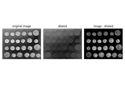
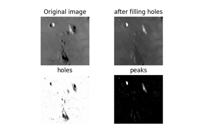
- skimage.morphology.remove_objects_by_distance(label_image, min_distance, *, priority=None, p_norm=2, spacing=None, out=None)[source]#
Remove objects, in specified order, until remaining are a minimum distance apart.
Remove labeled objects from an image until the remaining ones are spaced more than a given distance from one another. By default, smaller objects are removed first.
- Parameters:
- label_imagendarray of integers
An n-dimensional array containing object labels, e.g. as returned by
label(). A value of zero is considered background, all other object IDs must be positive integers.- min_distanceint or float
Remove objects whose distance to other objects is not greater than this positive value. Objects with a lower
priorityare removed first.- priorityndarray, optional
Defines the priority with which objects are removed. Expects a 1-dimensional array of length
np.amax(label_image) + 1that contains the priority for each object’s label at the respective index. Objects with a lower value are removed first until all remaining objects fulfill the distance requirement. If not given, priority is given to objects with a higher number of samples and their label value second.- p_normint or float, optional
The Minkowski distance of order p, used to calculate the distance between objects. The default
2corresponds to the Euclidean distance,1to the “Manhattan” distance, andnp.infto the Chebyshev distance.- spacingsequence of float, optional
The pixel spacing along each axis of
label_image. If not specified, a grid spacing of unity (1) is implied.- outndarray, optional
Array of the same shape and dtype as
image, into which the output is placed. By default, a new array is created.
- Returns:
- outndarray
Array of the same shape as
label_image, for which objects that violate themin_distancecondition were removed.
See also
skimage.morphology.remove_small_objectsRemove objects smaller than the specified size.
skimage.morphology.remove_small_holesRemove holes smaller than the specified size.
Notes
The basic steps of this algorithm work as follows:
Find the indices for of all given objects and separate them depending on if they point to an object’s border or not.
Sort indices by their label value, ensuring that indices which point to the same object are next to each other. This optimization allows finding all parts of an object, simply by stepping to the neighboring indices.
Sort boundary indices by
priority. Use a stable-sort to preserve the ordering from the previous sorting step. Ifpriorityis not given, usenumpy.bincount()as a fallback.Construct a
scipy.spatial.cKDTreefrom the boundary indices.Iterate across boundary indices in priority-sorted order, and query the kd-tree for objects that are too close. Remove ones that are and don’t take them into account when evaluating other objects later on.
The performance of this algorithm depends on the number of samples in
label_imagethat belong to an object’s border.Examples
>>> import skimage as ski
>>> ski.morphology.remove_objects_by_distance(np.array([2, 0, 1, 1]), 2)
array([0, 0, 1, 1])
>>> ski.morphology.remove_objects_by_distance(
...     np.array([2, 0, 1, 1]), 2, priority=np.array([0, 1, 9])
... )
array([2, 0, 0, 0])
>>> label_image = np.array(
...     [[8, 0, 0, 0, 0, 0, 0, 0, 0, 9, 9],
...      [8, 8, 8, 0, 0, 0, 0, 0, 0, 9, 9],
...      [0, 0, 0, 0, 0, 0, 0, 0, 9, 0, 0],
...      [0, 0, 0, 0, 0, 0, 0, 0, 0, 0, 0],
...      [0, 0, 3, 0, 0, 0, 1, 0, 0, 0, 0],
...      [2, 0, 0, 0, 0, 1, 0, 0, 0, 0, 0],
...      [0, 0, 0, 0, 0, 1, 0, 0, 0, 0, 0],
...      [0, 0, 0, 0, 0, 0, 0, 0, 0, 7, 7]]
... )
>>> ski.morphology.remove_objects_by_distance(
...     label_image, min_distance=3
... )
array([[8, 0, 0, 0, 0, 0, 0, 0, 0, 9, 9],
       [8, 8, 8, 0, 0, 0, 0, 0, 0, 9, 9],
       [0, 0, 0, 0, 0, 0, 0, 0, 9, 0, 0],
       [0, 0, 0, 0, 0, 0, 0, 0, 0, 0, 0],
       [0, 0, 0, 0, 0, 0, 0, 0, 0, 0, 0],
       [2, 0, 0, 0, 0, 0, 0, 0, 0, 0, 0],
       [0, 0, 0, 0, 0, 0, 0, 0, 0, 0, 0],
       [0, 0, 0, 0, 0, 0, 0, 0, 0, 7, 7]])

- skimage.morphology.remove_small_holes(ar, area_threshold=<DEPRECATED>, connectivity=1, *, max_size=64, out=None)[source]#
Remove contiguous holes smaller than the specified size.
- Parameters:
- arndarray (arbitrary shape, int or bool type)
The array containing the connected components of interest.
- max_sizeint, optional (default: 64)
Remove holes whose contiguous area (or volume, in N-D) contains this number of pixels or fewer.
Added in version 0.26: To make the naming clearer, replaces deprecated
area_thresholdwhich only removed holes strictly smaller than its size.- connectivityint, {1, 2, …, ar.ndim}, optional (default: 1)
The connectivity defining the neighborhood of a pixel.
- outndarray
Array of the same shape as
arand bool dtype, into which the output is placed. By default, a new array is created.
- Returns:
- outndarray, same shape and type as input
ar The input array with small holes within connected components removed.
- outndarray, same shape and type as input
- Other Parameters:
- area_thresholdDEPRECATED
Deprecated in favor of
max_size.Deprecated since version 0.26.0.
- Raises:
- TypeError
If the input array is of an invalid type, such as float or string.
- ValueError
If the input array contains negative values.
Notes
If the array type is int, it is assumed that it contains already-labeled objects. The labels are not kept in the output image (this function always outputs a bool image). It is suggested that labeling is completed after using this function.
Examples
>>> from skimage import morphology
>>> a = np.array([[1, 1, 1, 1, 1, 0],
...               [1, 1, 1, 0, 1, 0],
...               [1, 0, 0, 1, 1, 0],
...               [1, 1, 1, 1, 1, 0]], bool)
>>> b = morphology.remove_small_holes(a, max_size=1)
>>> b
array([[ True,  True,  True,  True,  True, False],
       [ True,  True,  True,  True,  True, False],
       [ True, False, False,  True,  True, False],
       [ True,  True,  True,  True,  True, False]])
>>> c = morphology.remove_small_holes(a, max_size=1, connectivity=2)
>>> c
array([[ True,  True,  True,  True,  True, False],
       [ True,  True,  True, False,  True, False],
       [ True, False, False,  True,  True, False],
       [ True,  True,  True,  True,  True, False]])
>>> d = morphology.remove_small_holes(a, max_size=1, out=a)
>>> d is a
True
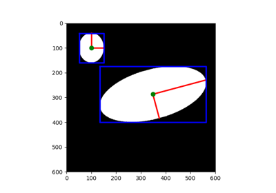
- skimage.morphology.remove_small_objects(ar, min_size=<DEPRECATED>, connectivity=1, *, max_size=64, out=None)[source]#
Remove objects smaller than the specified size.
Expects
arto be an array with labeled objects, and removes objects smaller than or equal tomax_size. Ifaris bool, the image is first labeled. This leads to potentially different behavior for bool vs. 0-and-1 arrays.- Parameters:
- arndarray (arbitrary shape, int or bool type)
The array containing the objects of interest. If the array type is int, the ints must be non-negative.
- max_sizeint, optional (default: 64)
Remove objects whose contiguous area (or volume, in N-D) contains this number of pixels or fewer.
Added in version 0.26: To make the naming clearer, replaces deprecated
min_sizewhich only removed objects strictly smaller than its size.- connectivityint, {1, 2, …, ar.ndim}, optional (default: 1)
The connectivity defining the neighborhood of a pixel. Used during labelling if
aris bool.- outndarray
Array of the same shape as
ar, into which the output is placed. By default, a new array is created.
- Returns:
- outndarray, same shape and type as input
ar The input array with small connected components removed.
- outndarray, same shape and type as input
- Other Parameters:
- min_sizeDEPRECATED
Deprecated in favor of
max_size.Deprecated since version 0.26.0.
- Raises:
- TypeError
If the input array is of an invalid type, such as float or string.
- ValueError
If the input array contains negative values.
Examples
>>> from skimage import morphology
>>> a = np.array([[0, 0, 0, 1, 0],
...               [1, 1, 1, 0, 0],
...               [1, 1, 1, 0, 1]], bool)
>>> b = morphology.remove_small_objects(a, max_size=5)
>>> b
array([[False, False, False, False, False],
       [ True,  True,  True, False, False],
       [ True,  True,  True, False, False]])
>>> c = morphology.remove_small_objects(a, max_size=6, connectivity=2)
>>> c
array([[False, False, False,  True, False],
       [ True,  True,  True, False, False],
       [ True,  True,  True, False, False]])
>>> d = morphology.remove_small_objects(a, max_size=5, out=a)
>>> d is a
True
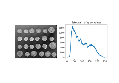
Comparing edge-based and region-based segmentation
Comparing edge-based and region-based segmentation
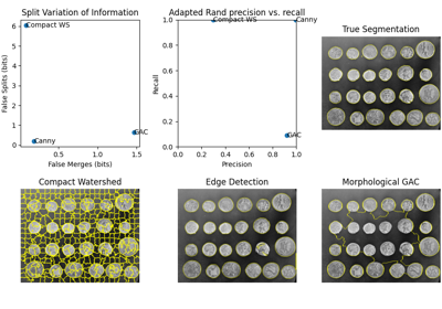
- skimage.morphology.skeletonize(image, *, method=None)[source]#
Compute the skeleton of the input image via thinning.
- Parameters:
- image(M, N[, P]) ndarray of bool or int
The image containing the objects to be skeletonized. Each connected component in the image is reduced to a single-pixel wide skeleton. The image is binarized prior to thinning; thus, adjacent objects of different intensities are considered as one. Zero or
Falsevalues represent the background, nonzero orTruevalues – foreground.- method{‘zhang’, ‘lee’}, optional
Which algorithm to use. Zhang’s algorithm [Zha84] only works for 2D images, and is the default for 2D. Lee’s algorithm [Lee94] works for 2D or 3D images and is the default for 3D.
- Returns:
- skeleton(M, N[, P]) ndarray of bool
The thinned image.
See also
References
[Lee94]T.-C. Lee, R.L. Kashyap and C.-N. Chu, Building skeleton models via 3-D medial surface/axis thinning algorithms. Computer Vision, Graphics, and Image Processing, 56(6):462-478, 1994.
[Zha84]A fast parallel algorithm for thinning digital patterns, T. Y. Zhang and C. Y. Suen, Communications of the ACM, March 1984, Volume 27, Number 3.
Examples
>>> X, Y = np.ogrid[0:9, 0:9]
>>> ellipse = (1./3 * (X - 4)**2 + (Y - 4)**2 < 3**2).astype(bool)
>>> ellipse.view(np.uint8)
array([[0, 0, 0, 1, 1, 1, 0, 0, 0],
       [0, 0, 1, 1, 1, 1, 1, 0, 0],
       [0, 0, 1, 1, 1, 1, 1, 0, 0],
       [0, 0, 1, 1, 1, 1, 1, 0, 0],
       [0, 0, 1, 1, 1, 1, 1, 0, 0],
       [0, 0, 1, 1, 1, 1, 1, 0, 0],
       [0, 0, 1, 1, 1, 1, 1, 0, 0],
       [0, 0, 1, 1, 1, 1, 1, 0, 0],
       [0, 0, 0, 1, 1, 1, 0, 0, 0]], dtype=uint8)
>>> skel = skeletonize(ellipse)
>>> skel.view(np.uint8)
array([[0, 0, 0, 0, 0, 0, 0, 0, 0],
       [0, 0, 0, 0, 0, 0, 0, 0, 0],
       [0, 0, 0, 0, 0, 0, 0, 0, 0],
       [0, 0, 0, 0, 1, 0, 0, 0, 0],
       [0, 0, 0, 0, 1, 0, 0, 0, 0],
       [0, 0, 0, 0, 1, 0, 0, 0, 0],
       [0, 0, 0, 0, 1, 0, 0, 0, 0],
       [0, 0, 0, 0, 0, 0, 0, 0, 0],
       [0, 0, 0, 0, 0, 0, 0, 0, 0]], dtype=uint8)
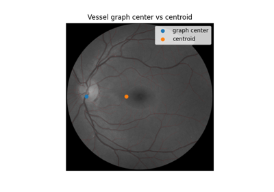
Use pixel graphs to find an object’s geodesic center
Use pixel graphs to find an object's geodesic center
- skimage.morphology.star(a, dtype=<class 'numpy.uint8'>)[source]#
Generates a star shaped footprint.
Start has 8 vertices and is an overlap of square of size
2*a + 1with its 45 degree rotated version. The slanted sides are 45 or 135 degrees to the horizontal axis.- Parameters:
- aint
Parameter deciding the size of the star structural element. The side of the square array returned is
2*a + 1 + 2*floor(a / 2).
- Returns:
- footprintndarray
The footprint where elements of the neighborhood are 1 and 0 otherwise.
- Other Parameters:
- dtypedata-type, optional
The data type of the footprint.
- skimage.morphology.thin(image, max_num_iter=None)[source]#
Perform morphological thinning of a binary image.
- Parameters:
- imagebinary (M, N) ndarray
The image to thin. If this input isn’t already a binary image, it gets converted into one: In this case, zero values are considered background (False), nonzero values are considered foreground (True).
- max_num_iterint, number of iterations, optional
Regardless of the value of this parameter, the thinned image is returned immediately if an iteration produces no change. If this parameter is specified it thus sets an upper bound on the number of iterations performed.
- Returns:
- outndarray of bool
Thinned image.
See also
Notes
This algorithm [1] works by making multiple passes over the image, removing pixels matching a set of criteria designed to thin connected regions while preserving eight-connected components and 2 x 2 squares [2]. In each of the two sub-iterations the algorithm correlates the intermediate skeleton image with a neighborhood mask, then looks up each neighborhood in a lookup table indicating whether the central pixel should be deleted in that sub-iteration.
References
[1]Z. Guo and R. W. Hall, “Parallel thinning with two-subiteration algorithms,” Comm. ACM, vol. 32, no. 3, pp. 359-373, 1989. DOI:10.1145/62065.62074
[2]Lam, L., Seong-Whan Lee, and Ching Y. Suen, “Thinning Methodologies-A Comprehensive Survey,” IEEE Transactions on Pattern Analysis and Machine Intelligence, Vol 14, No. 9, p. 879, 1992. DOI:10.1109/34.161346
Examples
>>> square = np.zeros((7, 7), dtype=bool)
>>> square[1:-1, 2:-2] = 1
>>> square[0, 1] =  1
>>> square.view(np.uint8)
array([[0, 1, 0, 0, 0, 0, 0],
       [0, 0, 1, 1, 1, 0, 0],
       [0, 0, 1, 1, 1, 0, 0],
       [0, 0, 1, 1, 1, 0, 0],
       [0, 0, 1, 1, 1, 0, 0],
       [0, 0, 1, 1, 1, 0, 0],
       [0, 0, 0, 0, 0, 0, 0]], dtype=uint8)
>>> skel = thin(square)
>>> skel.view(np.uint8)
array([[0, 1, 0, 0, 0, 0, 0],
       [0, 0, 1, 0, 0, 0, 0],
       [0, 0, 0, 1, 0, 0, 0],
       [0, 0, 0, 1, 0, 0, 0],
       [0, 0, 0, 1, 0, 0, 0],
       [0, 0, 0, 0, 0, 0, 0],
       [0, 0, 0, 0, 0, 0, 0]], dtype=uint8)
- skimage.morphology.white_tophat(image, footprint=None, out=None, *, mode='reflect', cval=0.0)[source]#
Return white top hat of an image.
The white top hat of an image is defined as the image minus its morphological opening. This operation returns the bright spots of the image that are smaller than the footprint.
- Parameters:
- imagendarray
Image array.
- footprintndarray or tuple, optional
The neighborhood expressed as a 2-D array of 1’s and 0’s. If None, use a cross-shaped footprint (connectivity=1). The footprint can also be provided as a sequence of smaller footprints as described in the notes below.
- outndarray, optional
The array to store the result of the morphology. If None is passed, a new array will be allocated.
- modestr, optional
The
modeparameter determines how the array borders are handled. Valid modes are: ‘reflect’, ‘constant’, ‘nearest’, ‘mirror’, ‘wrap’, ‘max’, ‘min’, or ‘ignore’. Seeskimage.morphology.opening(). Default is ‘reflect’.- cvalscalar, optional
Value to fill past edges of input if
modeis ‘constant’. Default is 0.0.Added in version 0.23:
modeandcvalwere added in 0.23.
- Returns:
- outarray, same shape and type as
image The result of the morphological white top hat.
- outarray, same shape and type as
See also
Notes
The footprint can also be a provided as a sequence of 2-tuples where the first element of each 2-tuple is a footprint ndarray and the second element is an integer describing the number of times it should be iterated. For example
footprint=[(np.ones((9, 1)), 1), (np.ones((1, 9)), 1)]would apply a 9x1 footprint followed by a 1x9 footprint resulting in a net effect that is the same asfootprint=np.ones((9, 9)), but with lower computational cost. Most of the builtin footprints such asskimage.morphology.disk()provide an option to automatically generate a footprint sequence of this type.References
Examples
>>> # Subtract gray background from bright peak
>>> import numpy as np
>>> from skimage.morphology import footprint_rectangle
>>> bright_on_gray = np.array([[2, 3, 3, 3, 2],
...                            [3, 4, 5, 4, 3],
...                            [3, 5, 9, 5, 3],
...                            [3, 4, 5, 4, 3],
...                            [2, 3, 3, 3, 2]], dtype=np.uint8)
>>> white_tophat(bright_on_gray, footprint_rectangle((3, 3)))
array([[0, 0, 0, 0, 0],
       [0, 0, 1, 0, 0],
       [0, 1, 5, 1, 0],
       [0, 0, 1, 0, 0],
       [0, 0, 0, 0, 0]], dtype=uint8)
Removing small objects in grayscale images with a top hat filter
Removing small objects in grayscale images with a top hat filter