Use rolling-ball algorithm for estimating background intensity

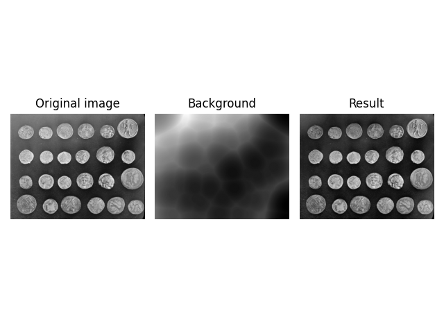
The rolling-ball algorithm estimates the background intensity of a grayscale image. It comes in useful, for instance, in case of uneven exposure, when subtracting the background is desirable. It is frequently used in biomedical image processing and was first proposed by Stanley R. Sternberg in 1983 [1].

The algorithm works as a filter: Think of the image as a surface that has unit-sized blocks stacked on top of each other in place of each pixel. The number of blocks, and hence surface height, is determined by the intensity of the pixel. To get the intensity of the background at a desired (pixel) position, we imagine submerging a ball under the surface at the desired position. Once it is completely covered by the blocks, the apex of the ball determines the intensity of the background at that position. We can then ‘roll’ this ball around below the surface to get the background values for the entire image. The larger the ball, the smoother the background.

scikit-image implements a generalized version of this rolling-ball algorithm, allowing you to work with n-dimensional images and to use not only balls, but other kernels as well. This way, you may directly filter RGB images or image stacks along any (or all) spatial dimensions.

[1]

Sternberg, Stanley R. “Biomedical image processing.” Computer 1 (1983): 22-34. DOI:10.1109/MC.1983.1654163

Classic rolling ball

In scikit-image, the implementation assumes that your image background has low intensity (dark), whereas the features have high intensity (bright). If this is not your case, you first have to invert the image—we give an example of that further on.

import matplotlib.pyplot as plt
import numpy as np

import pywt
import skimage as ski


def plot_result(image, background):
    fig, ax = plt.subplots(ncols=3)

    ax[0].imshow(image, cmap='gray')
    ax[0].set_title('Original image')
    ax[0].axis('off')

    ax[1].imshow(background, cmap='gray')
    ax[1].set_title('Background')
    ax[1].axis('off')

    ax[2].imshow(image - background, cmap='gray')
    ax[2].set_title('Result')
    ax[2].axis('off')

    fig.tight_layout()


image = ski.data.coins()

background = ski.restoration.rolling_ball(image)

plot_result(image, background)
plt.show()

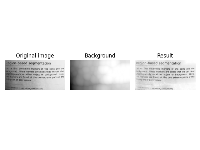
Bright background

If you have dark features on a bright background, you need to invert the image before passing it to the rolling-ball filter, and then invert the result. This can be accomplished as follows:

image = ski.data.page()
image_inverted = ski.util.invert(image)

background_inverted = ski.restoration.rolling_ball(image_inverted, radius=45)
filtered_image_inverted = image_inverted - background_inverted
filtered_image = ski.util.invert(filtered_image_inverted)
background = ski.util.invert(background_inverted)

fig, ax = plt.subplots(ncols=3)

ax[0].imshow(image, cmap='gray')
ax[0].set_title('Original image')
ax[0].axis('off')

ax[1].imshow(background, cmap='gray')
ax[1].set_title('Background')
ax[1].axis('off')

ax[2].imshow(filtered_image, cmap='gray')
ax[2].set_title('Result')
ax[2].axis('off')

fig.tight_layout()

plt.show()

Be careful not to fall victim to an integer underflow when subtracting a bright background. For example, this code looks correct, but may suffer from an underflow leading to unwanted artifacts. You can see this in the top right corner of the visualization.

image = ski.data.page()
image_inverted = ski.util.invert(image)

background_inverted = ski.restoration.rolling_ball(image_inverted, radius=45)
background = ski.util.invert(background_inverted)
underflow_image = image - background  # integer underflow occurs here

# correct subtraction
correct_image = ski.util.invert(image_inverted - background_inverted)

fig, ax = plt.subplots(ncols=2)

ax[0].imshow(underflow_image, cmap='gray')
ax[0].set_title('Background Removal with Underflow')
ax[0].axis('off')

ax[1].imshow(correct_image, cmap='gray')
ax[1].set_title('Correct Background Removal')
ax[1].axis('off')

fig.tight_layout()

plt.show()

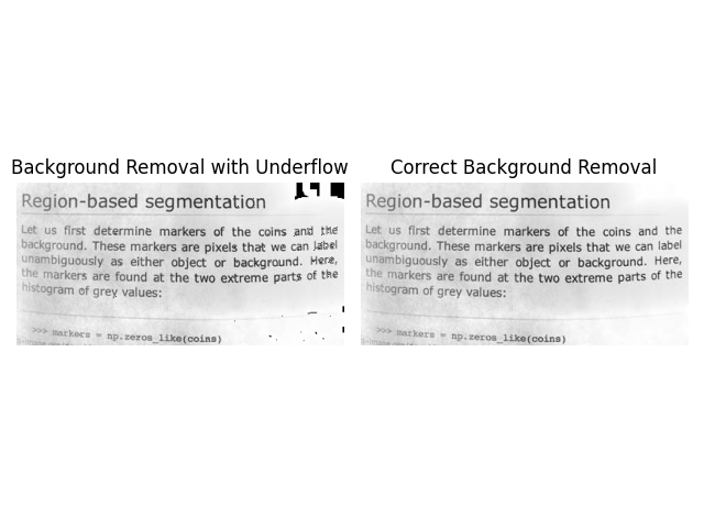
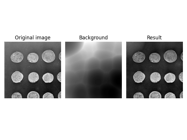
Image Datatypes

rolling_ball can handle datatypes other than np.uint8. You can pass them into the function in the same way.

image = ski.data.coins()[:200, :200].astype(np.uint16)

background = ski.restoration.rolling_ball(image, radius=70.5)
plot_result(image, background)
plt.show()

However, you need to be careful if you use floating point images that have been normalized to [0, 1]. In this case the ball will be much larger than the image intensity, which can lead to unexpected results.

image = ski.util.img_as_float(ski.data.coins()[:200, :200])

background = ski.restoration.rolling_ball(image, radius=70.5)
plot_result(image, background)
plt.show()

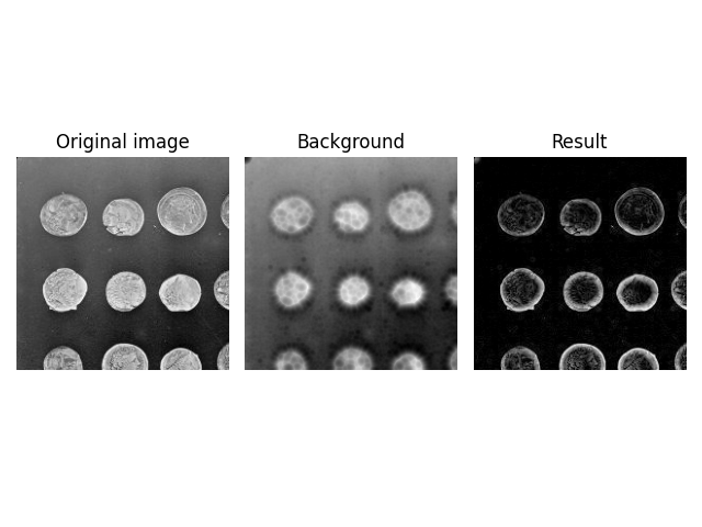
Because radius=70.5 is much larger than the maximum intensity of the image, the effective kernel size is reduced significantly, i.e., only a small cap (approximately radius=10) of the ball is rolled around in the image. You can find a reproduction of this strange effect in the Advanced Shapes section below.

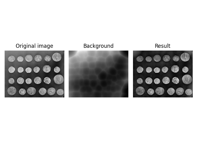
To get the expected result, you need to reduce the intensity of the kernel. This is done by specifying the kernel manually using the kernel argument.

Note: The radius is equal to the length of a semi-axis of an ellipsis, which is half a full axis. Hence, the kernel shape is multiplied by two.

normalized_radius = 70.5 / 255
image = ski.util.img_as_float(ski.data.coins())
kernel = ski.restoration.ellipsoid_kernel((70.5 * 2, 70.5 * 2), normalized_radius * 2)

background = ski.restoration.rolling_ball(image, kernel=kernel)
plot_result(image, background)
plt.show()

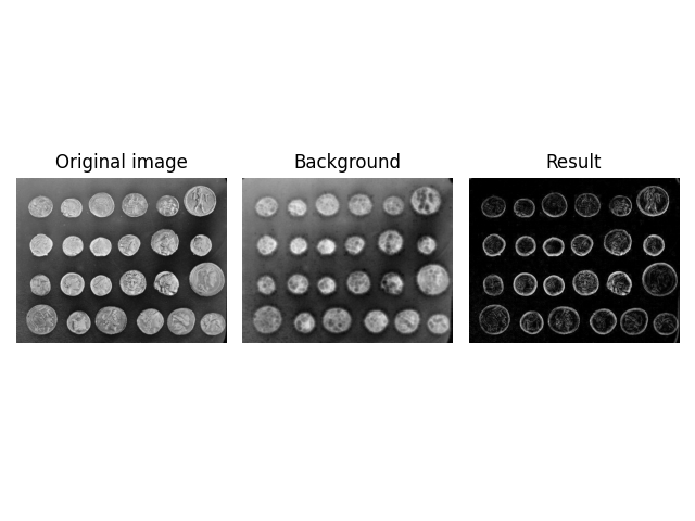
Advanced Shapes

By default, skimage.restoration.rolling_ball() uses a ball-shaped kernel (surprise). Sometimes, though, this can be too limiting—as in the example above, because the intensity dimension has a different scale compared to the spatial dimensions, or because the image dimensions may have different meanings (e.g., one could be a stack counter in an image stack).

To account for this, skimage.restoration.rolling_ball() has a kernel argument which allows you to specify the kernel to be used. A kernel must have the same dimensionality as the image (i.e., the same number of dimensions/axes). To help with its creation, two kernel implementations are provided: skimage.restoration.ball_kernel() specifies a ball-shaped kernel and is used as the default kernel; skimage.restoration.ellipsoid_kernel() specifies an ellipsoid-shaped kernel.

image = ski.data.coins()
kernel = ski.restoration.ellipsoid_kernel((70.5 * 2, 70.5 * 2), 70.5 * 2)

background = ski.restoration.rolling_ball(image, kernel=kernel)
plot_result(image, background)
plt.show()

You can also use skimage.restoration.ellipsoid_kernel() to recreate the previous, unexpected result and see that the effective (spatial) filter size was reduced.

image = ski.data.coins()
kernel = ski.restoration.ellipsoid_kernel((10 * 2, 10 * 2), 255 * 2)

background = ski.restoration.rolling_ball(image, kernel=kernel)
plot_result(image, background)
plt.show()

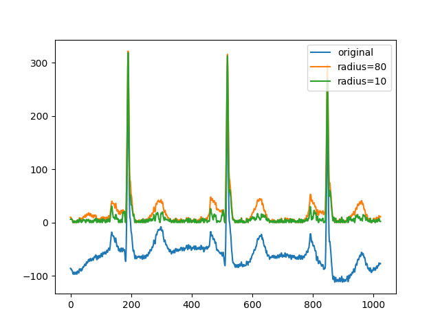
Higher Dimensions

Another interesting feature of skimage.restoration.rolling_ball() is that you can directly apply it to higher-dimensional images, e.g., a Z-stack of images obtained in confocal microscopy. The number of kernel dimensions must match that of image dimensions; in this case, the kernel is thus 3-dimensional.

image = ski.data.cells3d()[:, 1, ...]
kernel = ski.restoration.ellipsoid_kernel((1, 21, 21), 0.1)

background = ski.restoration.rolling_ball(image, kernel=kernel)

plot_result(image[30, ...], background[30, ...])
plt.show()

The above filter is actually applied to each image in the stack individually, since the kernel has size 1 along the Z axis.

To filter along all 3 dimensions at the same time, you must use sizes greater than 1 along all 3 dimensions.

Change the first line in the above code block.

 kernel = ski.restoration.ellipsoid_kernel((5, 21, 21), 0.1)

Another possibility is to filter individual pixels only along the planar (Z) axis.

This change here will show a lot more clearly in the result.

 kernel = ski.restoration.ellipsoid_kernel((100, 1, 1), 0.1)

1D Signal Filtering

As another example of the n-dimensional feature of rolling_ball, we show an implementation for 1D data. Here, we are interested in removing the background signal of an ECG waveform to detect prominent peaks (higher values than the local baseline). Smoother peaks can be removed with smaller values of the radius.

x = pywt.data.ecg()
background = ski.restoration.rolling_ball(x, radius=80)
background2 = ski.restoration.rolling_ball(x, radius=10)
plt.figure()
plt.plot(x, label='original')
plt.plot(x - background, label='radius=80')
plt.plot(x - background2, label='radius=10')
plt.legend()
plt.show()