Gabors / Primary Visual Cortex “Simple Cells” from an Image

How to build a (bio-plausible) sparse dictionary (or ‘codebook’, or ‘filterbank’) for e.g. image classification without any fancy math and with just standard python scientific libraries?

Please find below a short answer ;-)

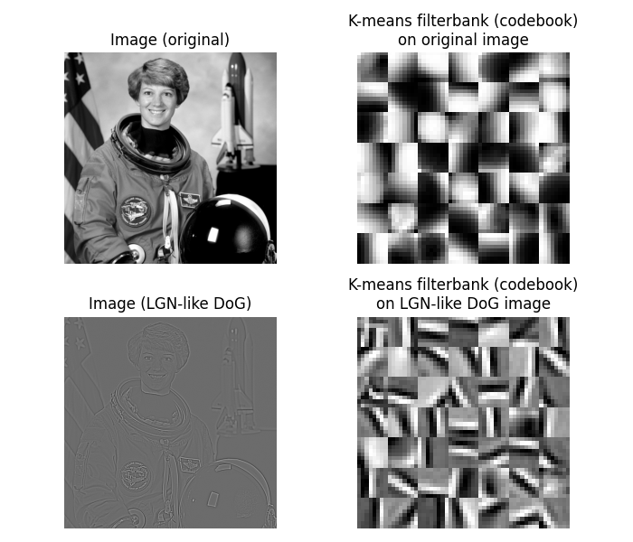
This simple example shows how to get Gabor-like filters [1] using just a simple image. In our example, we use a photograph of the astronaut Eileen Collins. Gabor filters are good approximations of the “Simple Cells” [2] receptive fields [3] found in the mammalian primary visual cortex (V1) (for details, see e.g. the Nobel-prize winning work of Hubel & Wiesel done in the 60s [4] [5]).

Here we use McQueen’s ‘kmeans’ algorithm [6], as a simple biologically plausible hebbian-like learning rule and we apply it (a) to patches of the original image (retinal projection), and (b) to patches of an LGN-like [7] image using a simple difference of gaussians (DoG) approximation.

Enjoy ;-) And keep in mind that getting Gabors on natural image patches is not rocket science.

[1]

https://en.wikipedia.org/wiki/Gabor_filter

[2]

https://en.wikipedia.org/wiki/Simple_cell

[3]

https://en.wikipedia.org/wiki/Receptive_field

[4]

D. H. Hubel and T. N., Wiesel Receptive Fields of Single Neurones in the Cat’s Striate Cortex, J. Physiol. pp. 574-591 (148) 1959

[5]

D. H. Hubel and T. N., Wiesel Receptive Fields, Binocular Interaction, and Functional Architecture in the Cat’s Visual Cortex, J. Physiol. 160 pp. 106-154 1962

[6]

https://en.wikipedia.org/wiki/K-means_clustering

[7]

https://en.wikipedia.org/wiki/Lateral_geniculate_nucleus

/home/runner/work/scikit-image/scikit-image/doc/examples/features_detection/plot_gabors_from_astronaut.py:57: UserWarning:

One of the clusters is empty. Re-run kmeans with a different initialization.

from scipy.cluster.vq import kmeans2
from scipy import ndimage as ndi
import matplotlib.pyplot as plt

from skimage import data
from skimage import color
from skimage.util.shape import view_as_windows
from skimage.util import montage

patch_shape = 8, 8
n_filters = 49

astro = color.rgb2gray(data.astronaut())

# -- filterbank1 on original image
patches1 = view_as_windows(astro, patch_shape)
patches1 = patches1.reshape(-1, patch_shape[0] * patch_shape[1])[::8]
fb1, _ = kmeans2(patches1, n_filters, minit='points')
fb1 = fb1.reshape((-1,) + patch_shape)
fb1_montage = montage(fb1, rescale_intensity=True)

# -- filterbank2 LGN-like image
astro_dog = ndi.gaussian_filter(astro, 0.5) - ndi.gaussian_filter(astro, 1)
patches2 = view_as_windows(astro_dog, patch_shape)
patches2 = patches2.reshape(-1, patch_shape[0] * patch_shape[1])[::8]
fb2, _ = kmeans2(patches2, n_filters, minit='points')
fb2 = fb2.reshape((-1,) + patch_shape)
fb2_montage = montage(fb2, rescale_intensity=True)

# -- plotting
fig, axes = plt.subplots(2, 2, figsize=(7, 6))
ax = axes.ravel()

ax[0].imshow(astro, cmap=plt.cm.gray)
ax[0].set_title("Image (original)")

ax[1].imshow(fb1_montage, cmap=plt.cm.gray)
ax[1].set_title("K-means filterbank (codebook)\non original image")

ax[2].imshow(astro_dog, cmap=plt.cm.gray)
ax[2].set_title("Image (LGN-like DoG)")

ax[3].imshow(fb2_montage, cmap=plt.cm.gray)
ax[3].set_title("K-means filterbank (codebook)\non LGN-like DoG image")

for a in ax.ravel():
    a.axis('off')

fig.tight_layout()
plt.show()