Estimate anisotropy in a 3D microscopy image

In this tutorial, we compute the structure tensor of a 3D image. For a general introduction to 3D image processing, please refer to Explore 3D images (of cells). The data we use here are sampled from an image of kidney tissue obtained by confocal fluorescence microscopy (more details at [1] under kidney-tissue-fluorescence.tif).

[1]

scikit-image/data/#data

import matplotlib.pyplot as plt
import numpy as np
import plotly.express as px
import plotly.io

from skimage import data, feature

Load image

This biomedical image is available through scikit-image’s data registry.

data = data.kidney()

What exactly are the shape and size of our 3D multichannel image?

print(f'number of dimensions: {data.ndim}')
print(f'shape: {data.shape}')
print(f'dtype: {data.dtype}')

number of dimensions: 4
shape: (16, 512, 512, 3)
dtype: uint16

For the purposes of this tutorial, we shall consider only the second color channel, which leaves us with a 3D single-channel image. What is the range of values?

n_plane, n_row, n_col, n_chan = data.shape
v_min, v_max = data[:, :, :, 1].min(), data[:, :, :, 1].max()
print(f'range: ({v_min}, {v_max})')

range: (68, 4095)

Let us visualize the middle slice of our 3D image.

fig1 = px.imshow(
    data[n_plane // 2, :, :, 1],
    zmin=v_min,
    zmax=v_max,
    labels={'x': 'col', 'y': 'row', 'color': 'intensity'},
)

plotly.io.show(fig1)

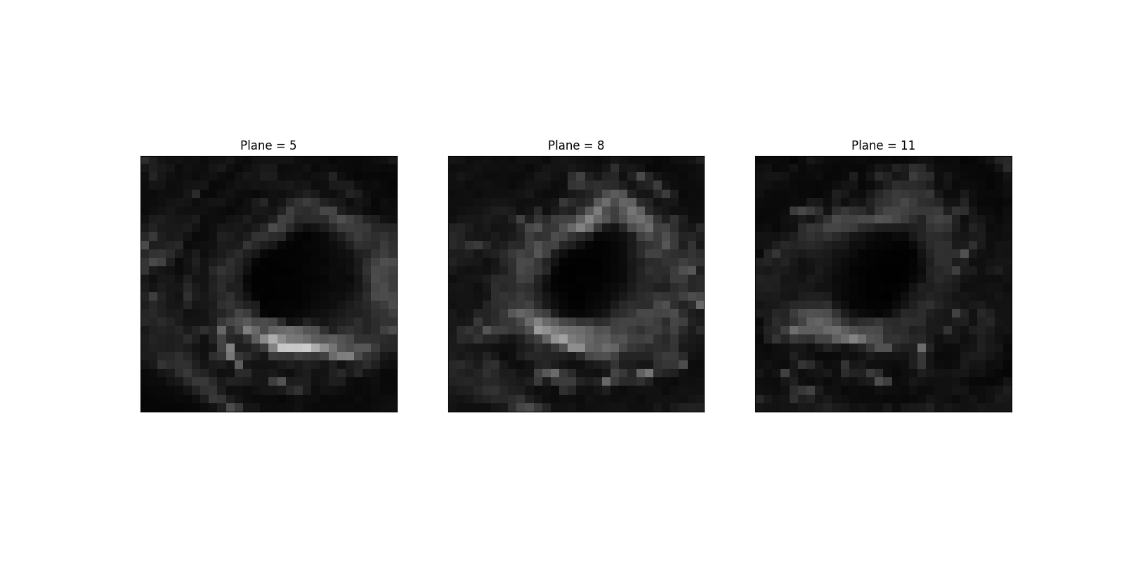
Let us pick a specific region, which shows relative X-Y isotropy. In contrast, the gradient is quite different (and, for that matter, weak) along Z.

sample = data[5:13, 380:410, 370:400, 1]
step = 3
cols = sample.shape[0] // step + 1
_, axes = plt.subplots(nrows=1, ncols=cols, figsize=(16, 8))

for it, (ax, image) in enumerate(zip(axes.flatten(), sample[::step])):
    ax.imshow(image, cmap='gray', vmin=v_min, vmax=v_max)
    ax.set_title(f'Plane = {5 + it * step}')
    ax.set_xticks([])
    ax.set_yticks([])

To view the sample data in 3D, run the following code:

import plotly.graph_objects as go

(n_Z, n_Y, n_X) = sample.shape
Z, Y, X = np.mgrid[:n_Z, :n_Y, :n_X]

fig = go.Figure(
    data=go.Volume(
        x=X.flatten(),
        y=Y.flatten(),
        z=Z.flatten(),
        value=sample.flatten(),
        opacity=0.5,
        slices_z=dict(show=True, locations=[4])
    )
)
fig.show()

Compute structure tensor

Let us visualize the bottom slice of our sample data and determine the typical size for strong variations. We shall use this size as the ‘width’ of the window function.

fig2 = px.imshow(
    sample[0, :, :],
    zmin=v_min,
    zmax=v_max,
    labels={'x': 'col', 'y': 'row', 'color': 'intensity'},
    title='Interactive view of bottom slice of sample data.',
)

plotly.io.show(fig2)

About the brightest region (i.e., at row ~ 22 and column ~ 17), we can see variations (and, hence, strong gradients) over 2 or 3 (resp. 1 or 2) pixels across columns (resp. rows). We may thus choose, say, sigma = 1.5 for the window function. Alternatively, we can pass sigma on a per-axis basis, e.g., sigma = (1, 2, 3). Note that size 1 sounds reasonable along the first (Z, plane) axis, since the latter is of size 8 (13 - 5). Viewing slices in the X-Z or Y-Z planes confirms it is reasonable.

sigma = (1, 1.5, 2.5)
A_elems = feature.structure_tensor(sample, sigma=sigma)

We can then compute the eigenvalues of the structure tensor.

eigen = feature.structure_tensor_eigenvalues(A_elems)
eigen.shape

(3, 8, 30, 30)

Where is the largest eigenvalue?

coords = np.unravel_index(eigen.argmax(), eigen.shape)
assert coords[0] == 0  # by definition
coords

(0, 1, 22, 16)

Note

The reader may check how robust this result (coordinates (plane, row, column) = coords[1:]) is to varying sigma.

Let us view the spatial distribution of the eigenvalues in the X-Y plane where the maximum eigenvalue is found (i.e., Z = coords[1]).

fig3 = px.imshow(
    eigen[:, coords[1], :, :],
    facet_col=0,
    labels={'x': 'col', 'y': 'row', 'facet_col': 'rank'},
    title=f'Eigenvalues for plane Z = {coords[1]}.',
)

plotly.io.show(fig3)

We are looking at a local property. Let us consider a tiny neighborhood around the maximum eigenvalue in the above X-Y plane.

eigen[0, coords[1], coords[2] - 2 : coords[2] + 1, coords[3] - 2 : coords[3] + 1]

array([[0.05530323, 0.05929082, 0.06043806],
       [0.05922725, 0.06268274, 0.06354238],
       [0.06190861, 0.06685075, 0.06840962]])

If we examine the second-largest eigenvalues in this neighborhood, we can see that they have the same order of magnitude as the largest ones.

eigen[1, coords[1], coords[2] - 2 : coords[2] + 1, coords[3] - 2 : coords[3] + 1]

array([[0.03577746, 0.03577334, 0.03447714],
       [0.03819524, 0.04172036, 0.04323701],
       [0.03139592, 0.03587025, 0.03913327]])

In contrast, the third-largest eigenvalues are one order of magnitude smaller.

eigen[2, coords[1], coords[2] - 2 : coords[2] + 1, coords[3] - 2 : coords[3] + 1]

array([[0.00337661, 0.00306529, 0.00276288],
       [0.0041869 , 0.00397519, 0.00375595],
       [0.00479742, 0.00462116, 0.00442455]])

Let us visualize the slice of sample data in the X-Y plane where the maximum eigenvalue is found.

fig4 = px.imshow(
    sample[coords[1], :, :],
    zmin=v_min,
    zmax=v_max,
    labels={'x': 'col', 'y': 'row', 'color': 'intensity'},
    title=f'Interactive view of plane Z = {coords[1]}.',
)

plotly.io.show(fig4)

Let us visualize the slices of sample data in the X-Z (left) and Y-Z (right) planes where the maximum eigenvalue is found. The Z axis is the vertical axis in the subplots below. We can see the expected relative invariance along the Z axis (corresponding to longitudinal structures in the kidney tissue), especially in the Y-Z plane (longitudinal=1).

subplots = np.dstack((sample[:, coords[2], :], sample[:, :, coords[3]]))
fig5 = px.imshow(
    subplots, zmin=v_min, zmax=v_max, facet_col=2, labels={'facet_col': 'longitudinal'}
)

plotly.io.show(fig5)

As a conclusion, the region about voxel (plane, row, column) = coords[1:] is anisotropic in 3D: There is an order of magnitude between the third-largest eigenvalues on one hand, and the largest and second-largest eigenvalues on the other hand. We could see this at first glance in figure Eigenvalues for plane Z = 1.

The neighborhood in question is ‘somewhat isotropic’ in a plane (which, here, would be relatively close to the X-Y plane): There is a factor of less than 2 between the second-largest and largest eigenvalues. This description is compatible with what we are seeing in the image, i.e., a stronger gradient across a direction (which, here, would be relatively close to the row axis) and a weaker gradient perpendicular to it.

In an ellipsoidal representation of the 3D structure tensor [2], we would get the pancake situation.

[2]

https://en.wikipedia.org/wiki/Structure_tensor#Interpretation_2