Morphological Filtering

Morphological image processing is a collection of non-linear operations related to the shape or morphology of features in an image, such as boundaries, skeletons, etc. In any given technique, we probe an image with a small shape or template called a structuring element, which defines the region of interest or neighborhood around a pixel.

In this document we outline the following basic morphological operations:

1. Erosion

2. Dilation

3. Opening

4. Closing

5. White Tophat

6. Black Tophat

7. Skeletonize

8. Convex Hull

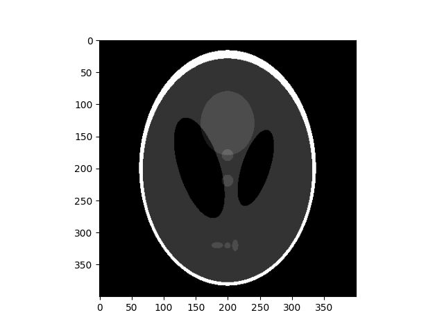
To get started, let’s load an image using io.imread. Note that morphology functions only work on gray-scale or binary images, so we set as_gray=True.

import matplotlib.pyplot as plt
from skimage import data
from skimage.util import img_as_ubyte

orig_phantom = img_as_ubyte(data.shepp_logan_phantom())
fig, ax = plt.subplots()
ax.imshow(orig_phantom, cmap=plt.cm.gray)

<matplotlib.image.AxesImage object at 0x7fc9b0fe0d10>

Let’s also define a convenience function for plotting comparisons:

def plot_comparison(original, filtered, filter_name):
    fig, (ax1, ax2) = plt.subplots(ncols=2, figsize=(8, 4), sharex=True, sharey=True)
    ax1.imshow(original, cmap=plt.cm.gray)
    ax1.set_title('original')
    ax1.set_axis_off()
    ax2.imshow(filtered, cmap=plt.cm.gray)
    ax2.set_title(filter_name)
    ax2.set_axis_off()

Erosion

Morphological erosion sets a pixel at (i, j) to the minimum over all pixels in the neighborhood centered at (i, j). The structuring element, footprint, passed to erosion is a boolean array that describes this neighborhood. Below, we use disk to create a circular structuring element, which we use for most of the following examples.

from skimage.morphology import erosion, dilation, opening, closing, white_tophat  # noqa
from skimage.morphology import black_tophat, skeletonize, convex_hull_image  # noqa
from skimage.morphology import disk  # noqa

footprint = disk(6)
eroded = erosion(orig_phantom, footprint)
plot_comparison(orig_phantom, eroded, 'erosion')

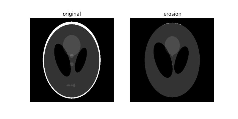
Notice how the white boundary of the image disappears or gets eroded as we increase the size of the disk. Also notice the increase in size of the two black ellipses in the center and the disappearance of the 3 light gray patches in the lower part of the image.

Dilation

Morphological dilation sets a pixel at (i, j) to the maximum over all pixels in the neighborhood centered at (i, j). Dilation enlarges bright regions and shrinks dark regions.

dilated = dilation(orig_phantom, footprint)
plot_comparison(orig_phantom, dilated, 'dilation')

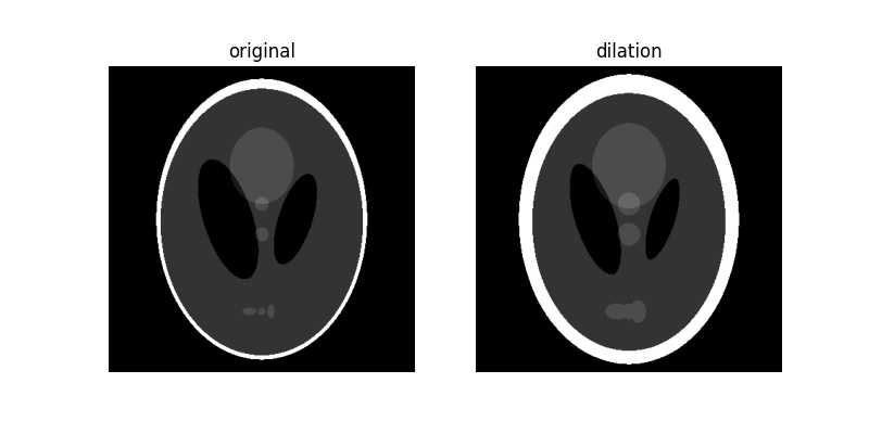
Notice how the white boundary of the image thickens, or gets dilated, as we increase the size of the disk. Also notice the decrease in size of the two black ellipses in the center, and the thickening of the light gray circle in the center and the 3 patches in the lower part of the image.

Opening

Morphological opening on an image is defined as an erosion followed by a dilation. Opening can remove small bright spots (i.e. “salt”) and connect small dark cracks.

opened = opening(orig_phantom, footprint)
plot_comparison(orig_phantom, opened, 'opening')

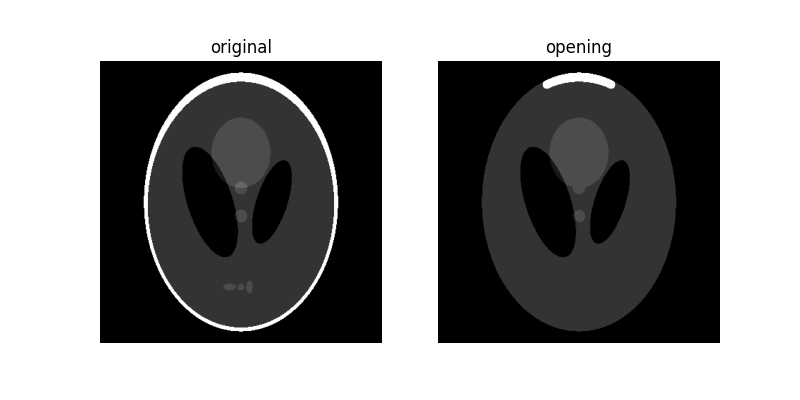
Since opening an image starts with an erosion operation, light regions that are smaller than the structuring element are removed. The dilation operation that follows ensures that light regions that are larger than the structuring element retain their original size. Notice how the light and dark shapes in the center retain their original thickness but the 3 lighter patches in the bottom get completely eroded. The size dependence is highlighted by the outer white ring: The parts of the ring thinner than the structuring element are completely erased, while the thicker region at the top retains its original thickness.

Closing

Morphological closing on an image is defined as a dilation followed by an erosion. Closing can remove small dark spots (i.e. “pepper”) and connect small bright cracks.

To illustrate this more clearly, let’s add a small crack to the white border:

phantom = orig_phantom.copy()
phantom[10:30, 200:210] = 0

closed = closing(phantom, footprint)
plot_comparison(phantom, closed, 'closing')

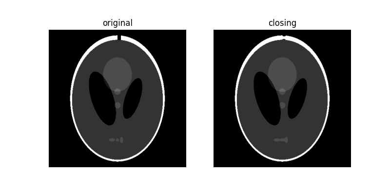
Since closing an image starts with a dilation operation, dark regions that are smaller than the structuring element are removed. The dilation operation that follows ensures that dark regions that are larger than the structuring element retain their original size. Notice how the white ellipses at the bottom get connected because of dilation, but other dark regions retain their original sizes. Also notice how the crack we added is mostly removed.

White tophat

The white_tophat of an image is defined as the image minus its morphological opening. This operation returns the bright spots of the image that are smaller than the structuring element.

To make things interesting, we’ll add bright and dark spots to the image:

phantom = orig_phantom.copy()
phantom[340:350, 200:210] = 255
phantom[100:110, 200:210] = 0

w_tophat = white_tophat(phantom, footprint)
plot_comparison(phantom, w_tophat, 'white tophat')

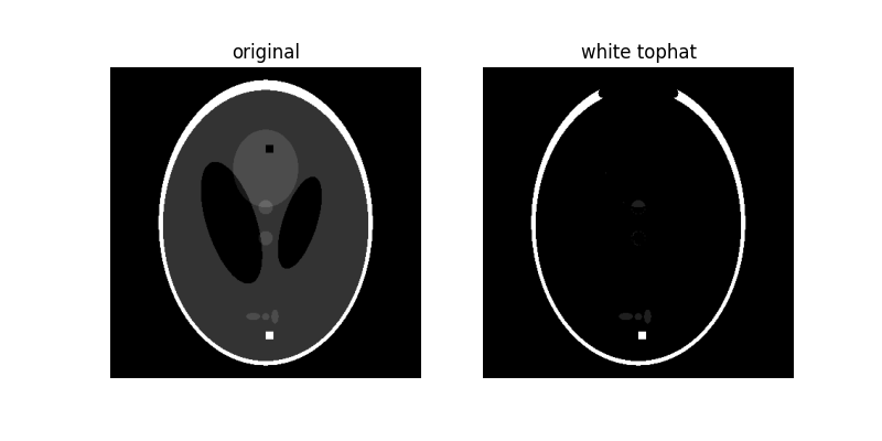
As you can see, the 10-pixel wide white square is highlighted since it is smaller than the structuring element. Also, the thin, white edges around most of the ellipse are retained because they’re smaller than the structuring element, but the thicker region at the top disappears.

Black tophat

The black_tophat of an image is defined as its morphological closing minus the original image. This operation returns the dark spots of the image that are smaller than the structuring element.

b_tophat = black_tophat(phantom, footprint)
plot_comparison(phantom, b_tophat, 'black tophat')

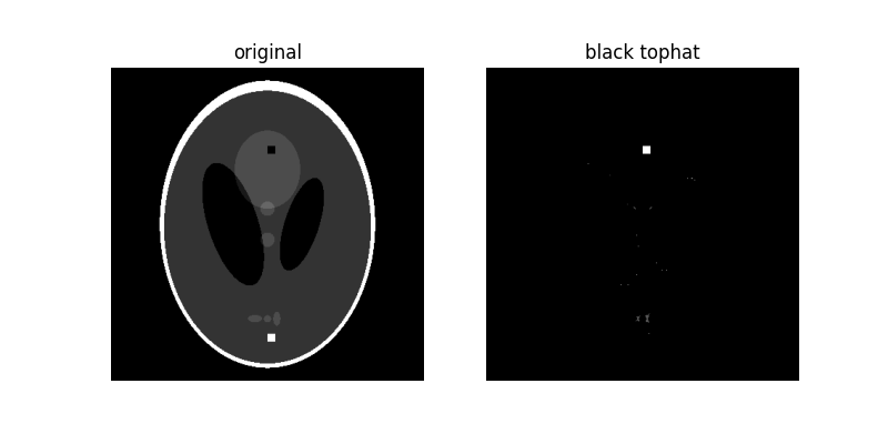
As you can see, the 10-pixel wide black square is highlighted since it is smaller than the structuring element.

Duality

As you should have noticed, many of these operations are simply the reverse of another operation. This duality can be summarized as follows:

1. Erosion <-> Dilation

2. Opening <-> Closing

3. White tophat <-> Black tophat

Skeletonize

Thinning is used to reduce each connected component in a binary image to a single-pixel wide skeleton. It is important to note that this is performed on binary images only.

horse = data.horse()

sk = skeletonize(horse == 0)
plot_comparison(horse, sk, 'skeletonize')

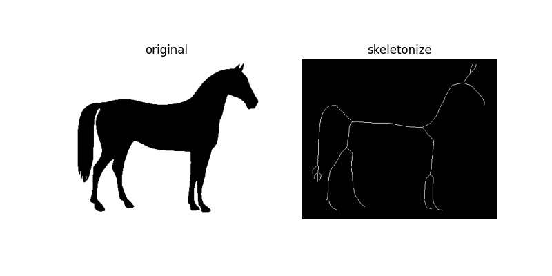
As the name suggests, this technique is used to thin the image to 1-pixel wide skeleton by applying thinning successively.

Convex hull

The convex_hull_image is the set of pixels included in the smallest convex polygon that surround all white pixels in the input image. Again note that this is also performed on binary images.

hull1 = convex_hull_image(horse == 0)
plot_comparison(horse, hull1, 'convex hull')

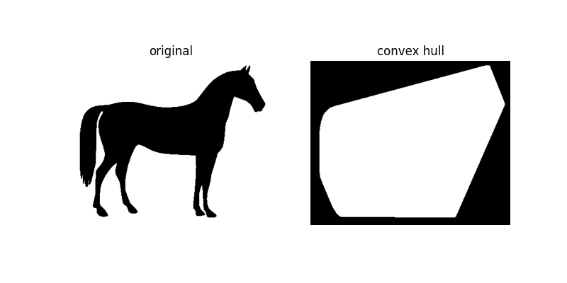
As the figure illustrates, convex_hull_image gives the smallest polygon which covers the white or True completely in the image.

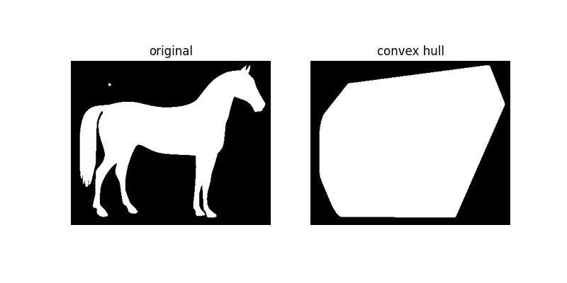
If we add a small grain to the image, we can see how the convex hull adapts to enclose that grain:

horse_mask = horse == 0
horse_mask[45:50, 75:80] = 1

hull2 = convex_hull_image(horse_mask)
plot_comparison(horse_mask, hull2, 'convex hull')

Additional Resources

1. MathWorks tutorial on morphological processing

2. Auckland university’s tutorial on Morphological Image Processing

3. https://en.wikipedia.org/wiki/Mathematical_morphology

plt.show()