Measure fluorescence intensity at the nuclear envelope

This example reproduces a well-established workflow in bioimage data analysis for measuring the fluorescence intensity localized to the nuclear envelope, in a time sequence of cell images (each with two channels and two spatial dimensions) which shows a process of protein re-localization from the cytoplasmic area to the nuclear envelope. This biological application was first presented by Andrea Boni and collaborators in [1]; it was used in a textbook by Kota Miura [2] as well as in other works ([3], [4]). In other words, we port this workflow from ImageJ Macro to Python with scikit-image.

[1]

Boni A, Politi AZ, Strnad P, Xiang W, Hossain MJ, Ellenberg J (2015) “Live imaging and modeling of inner nuclear membrane targeting reveals its molecular requirements in mammalian cells” J Cell Biol 209(5):705–720. ISSN: 0021-9525. DOI:10.1083/jcb.201409133

[2]

Miura K (2020) “Measurements of Intensity Dynamics at the Periphery of the Nucleus” in: Miura K, Sladoje N (eds) Bioimage Data Analysis Workflows. Learning Materials in Biosciences. Springer, Cham. DOI:10.1007/978-3-030-22386-1_2

[3]

Klemm A (2020) “ImageJ/Fiji Macro Language” NEUBIAS Academy Online Course: https://www.youtube.com/watch?v=o8tfkdcd3DA

[4]

Vorkel D and Haase R (2020) “GPU-accelerating ImageJ Macro image processing workflows using CLIJ” https://arxiv.org/abs/2008.11799

import matplotlib.pyplot as plt
import numpy as np
import plotly.io
import plotly.express as px
from scipy import ndimage as ndi

from skimage import filters, measure, morphology, segmentation
from skimage.data import protein_transport

We start with a single cell/nucleus to construct the workflow.

image_sequence = protein_transport()

print(f'shape: {image_sequence.shape}')

shape: (15, 2, 180, 183)

The dataset is a 2D image stack with 15 frames (time points) and 2 channels.

vmin, vmax = 0, image_sequence.max()

fig = px.imshow(
    image_sequence,
    facet_col=1,
    animation_frame=0,
    zmin=vmin,
    zmax=vmax,
    binary_string=True,
    labels={'animation_frame': 'time point', 'facet_col': 'channel'},
)
plotly.io.show(fig)

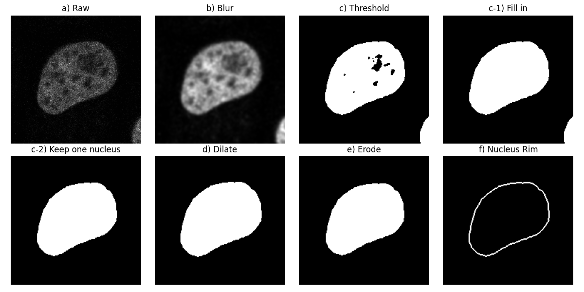
To begin with, let us consider the first channel of the first image (step a) in the figure below).

image_t_0_channel_0 = image_sequence[0, 0, :, :]

Segment the nucleus rim

Let us apply a Gaussian low-pass filter to this image in order to smooth it (step b)). Next, we segment the nuclei, finding the threshold between the background and foreground with Otsu’s method: We get a binary image (step c)). We then fill the holes in the objects (step c-1)).

smooth = filters.gaussian(image_t_0_channel_0, sigma=1.5)

thresh_value = filters.threshold_otsu(smooth)
thresh = smooth > thresh_value

fill = ndi.binary_fill_holes(thresh)

Following the original workflow, let us remove objects which touch the image border (step c-2)). Here, we can see that part of another nucleus was touching the bottom right-hand corner.

clear = segmentation.clear_border(fill)
clear.dtype

dtype('bool')

We compute both the morphological dilation of this binary image (step d)) and its morphological erosion (step e)).

dilate = morphology.binary_dilation(clear)

erode = morphology.binary_erosion(clear)

Finally, we subtract the eroded from the dilated to get the nucleus rim (step f)). This is equivalent to selecting the pixels which are in dilate, but not in erode:

mask = np.logical_and(dilate, ~erode)

Let us visualize these processing steps in a sequence of subplots.

fig, ax = plt.subplots(2, 4, figsize=(12, 6), sharey=True)

ax[0, 0].imshow(image_t_0_channel_0, cmap=plt.cm.gray)
ax[0, 0].set_title('a) Raw')

ax[0, 1].imshow(smooth, cmap=plt.cm.gray)
ax[0, 1].set_title('b) Blur')

ax[0, 2].imshow(thresh, cmap=plt.cm.gray)
ax[0, 2].set_title('c) Threshold')

ax[0, 3].imshow(fill, cmap=plt.cm.gray)
ax[0, 3].set_title('c-1) Fill in')

ax[1, 0].imshow(clear, cmap=plt.cm.gray)
ax[1, 0].set_title('c-2) Keep one nucleus')

ax[1, 1].imshow(dilate, cmap=plt.cm.gray)
ax[1, 1].set_title('d) Dilate')

ax[1, 2].imshow(erode, cmap=plt.cm.gray)
ax[1, 2].set_title('e) Erode')

ax[1, 3].imshow(mask, cmap=plt.cm.gray)
ax[1, 3].set_title('f) Nucleus Rim')

for a in ax.ravel():
    a.set_axis_off()

fig.tight_layout()

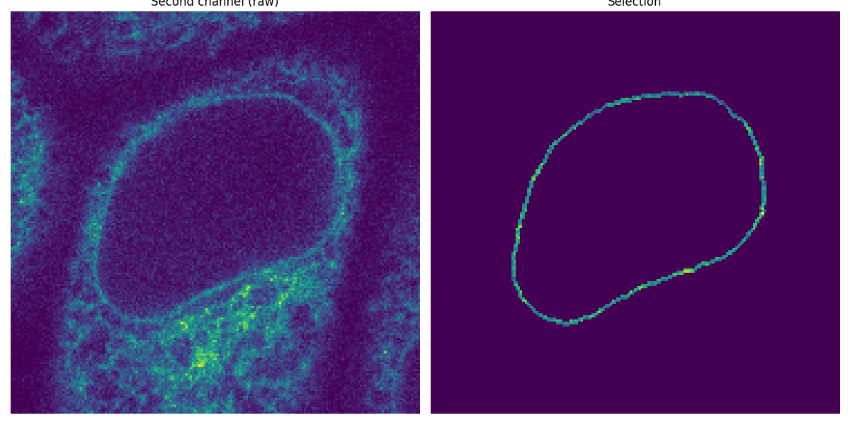
Apply the segmented rim as a mask

Now that we have segmented the nuclear membrane in the first channel, we use it as a mask to measure the intensity in the second channel.

image_t_0_channel_1 = image_sequence[0, 1, :, :]
selection = np.where(mask, image_t_0_channel_1, 0)

fig, (ax0, ax1) = plt.subplots(1, 2, figsize=(12, 6), sharey=True)

ax0.imshow(image_t_0_channel_1)
ax0.set_title('Second channel (raw)')
ax0.set_axis_off()

ax1.imshow(selection)
ax1.set_title('Selection')
ax1.set_axis_off()

fig.tight_layout()

Measure the total intensity

The mean intensity is readily available as a region property in a labeled image.

props = measure.regionprops_table(
    mask.astype(np.uint8),
    intensity_image=image_t_0_channel_1,
    properties=('label', 'area', 'intensity_mean'),
)

We may want to check that the value for the total intensity

selection.sum()

28350

can be recovered from:

props['area'] * props['intensity_mean']

array([28350.])

Process the entire image sequence

Instead of iterating the workflow for each time point, we process the multidimensional dataset directly (except for the thresholding step). Indeed, most scikit-image functions support nD images.

n_z = image_sequence.shape[0]  # number of frames

smooth_seq = filters.gaussian(image_sequence[:, 0, :, :], sigma=(0, 1.5, 1.5))
thresh_values = [filters.threshold_otsu(s) for s in smooth_seq[:]]
thresh_seq = [smooth_seq[k, ...] > val for k, val in enumerate(thresh_values)]

Alternatively, we could compute thresh_values without using a list comprehension, by reshaping smooth_seq to make it 2D (where the first dimension still corresponds to time points, but the second and last dimension now contains all pixel values), and applying the thresholding function on the image sequence along its second axis:

thresh_values = np.apply_along_axis(filters.threshold_otsu,
                                    axis=1,
                                    arr=smooth_seq.reshape(n_z, -1))

We use the following flat structuring element for morphological computations (np.newaxis is used to prepend an axis of size 1 for time):

footprint = ndi.generate_binary_structure(2, 1)[np.newaxis, ...]
footprint

array([[[False,  True, False],
        [ True,  True,  True],
        [False,  True, False]]])

This way, each frame is processed independently (pixels from consecutive frames are never spatial neighbors).

fill_seq = ndi.binary_fill_holes(thresh_seq, structure=footprint)

When clearing objects which touch the image border, we want to make sure that the bottom (first) and top (last) frames are not considered as borders. In this case, the only relevant border is the edge at the greatest (x, y) values. This can be seen in 3D by running the following code:

import plotly.graph_objects as go

sample = fill_seq
(n_Z, n_Y, n_X) = sample.shape
Z, Y, X = np.mgrid[:n_Z, :n_Y, :n_X]

fig = go.Figure(
    data=go.Volume(
        x=X.flatten(),
        y=Y.flatten(),
        z=Z.flatten(),
        value=sample.flatten(),
        opacity=0.5,
        slices_z=dict(show=True, locations=[n_z // 2])
    )
)
fig.show()

border_mask = np.ones_like(fill_seq)
border_mask[n_z // 2, -1, -1] = False
clear_seq = segmentation.clear_border(fill_seq, mask=border_mask)

dilate_seq = morphology.binary_dilation(clear_seq, footprint=footprint)
erode_seq = morphology.binary_erosion(clear_seq, footprint=footprint)
mask_sequence = np.logical_and(dilate_seq, ~erode_seq)

Let us give each mask (corresponding to each time point) a different label, running from 1 to 15. We use np.min_scalar_type to determine the minimum-size integer dtype needed to represent the number of time points:

label_dtype = np.min_scalar_type(n_z)
mask_sequence = mask_sequence.astype(label_dtype)
labels = np.arange(1, n_z + 1, dtype=label_dtype)
mask_sequence *= labels[:, np.newaxis, np.newaxis]

Let us compute the region properties of interest for all these labeled regions.

props = measure.regionprops_table(
    mask_sequence,
    intensity_image=image_sequence[:, 1, :, :],
    properties=('label', 'area', 'intensity_mean'),
)
np.testing.assert_array_equal(props['label'], np.arange(n_z) + 1)

fluorescence_change = [
    props['area'][i] * props['intensity_mean'][i] for i in range(n_z)
]

fluorescence_change /= fluorescence_change[0]  # normalization

fig, ax = plt.subplots()
ax.plot(fluorescence_change, 'rs')
ax.grid()
ax.set_xlabel('Time point')
ax.set_ylabel('Normalized total intensity')
ax.set_title('Change in fluorescence intensity at the nuclear envelope')
fig.tight_layout()

plt.show()

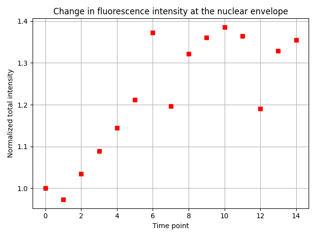
Reassuringly, we find the expected result: The total fluorescence intensity at the nuclear envelope increases 1.3-fold in the initial five time points, and then becomes roughly constant.