Note
Go to the end to download the full example code or to run this example in your browser via Binder.
Radon transform#
In computed tomography, the tomography reconstruction problem is to obtain a tomographic slice image from a set of projections [1]. A projection is formed by drawing a set of parallel rays through the 2D object of interest, assigning the integral of the object’s contrast along each ray to a single pixel in the projection. A single projection of a 2D object is one dimensional. To enable computed tomography reconstruction of the object, several projections must be acquired, each of them corresponding to a different angle between the rays with respect to the object. A collection of projections at several angles is called a sinogram, which is a linear transform of the original image.
The inverse Radon transform is used in computed tomography to reconstruct a 2D image from the measured projections (the sinogram). A practical, exact implementation of the inverse Radon transform does not exist, but there are several good approximate algorithms available.
As the inverse Radon transform reconstructs the object from a set of projections, the (forward) Radon transform can be used to simulate a tomography experiment.
This script performs the Radon transform to simulate a tomography experiment and reconstructs the input image based on the resulting sinogram formed by the simulation. Two methods for performing the inverse Radon transform and reconstructing the original image are compared: The Filtered Back Projection (FBP) and the Simultaneous Algebraic Reconstruction Technique (SART).
For further information on tomographic reconstruction, see:
The forward transform#
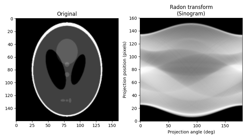
As our original image, we will use the Shepp-Logan phantom. When calculating the Radon transform, we need to decide how many projection angles we wish to use. As a rule of thumb, the number of projections should be about the same as the number of pixels there are across the object (to see why this is so, consider how many unknown pixel values must be determined in the reconstruction process and compare this to the number of measurements provided by the projections), and we follow that rule here. Below is the original image and its Radon transform, often known as its sinogram:
import numpy as np
import matplotlib.pyplot as plt

from skimage.data import shepp_logan_phantom
from skimage.transform import radon, rescale

image = shepp_logan_phantom()
image = rescale(image, scale=0.4, mode='reflect', channel_axis=None)

fig, (ax1, ax2) = plt.subplots(1, 2, figsize=(8, 4.5))

ax1.set_title("Original")
ax1.imshow(image, cmap=plt.cm.Greys_r)

theta = np.linspace(0.0, 180.0, max(image.shape), endpoint=False)
sinogram = radon(image, theta=theta)
dx, dy = 0.5 * 180.0 / max(image.shape), 0.5 / sinogram.shape[0]
ax2.set_title("Radon transform\n(Sinogram)")
ax2.set_xlabel("Projection angle (deg)")
ax2.set_ylabel("Projection position (pixels)")
ax2.imshow(
    sinogram,
    cmap=plt.cm.Greys_r,
    extent=(-dx, 180.0 + dx, -dy, sinogram.shape[0] + dy),
    aspect='auto',
)

fig.tight_layout()
plt.show()
Reconstruction with the Filtered Back Projection (FBP)#
The mathematical foundation of the filtered back projection is the Fourier
slice theorem [2]. It uses Fourier transform of the projection and
interpolation in Fourier space to obtain the 2D Fourier transform of the
image, which is then inverted to form the reconstructed image. The filtered
back projection is among the fastest methods of performing the inverse
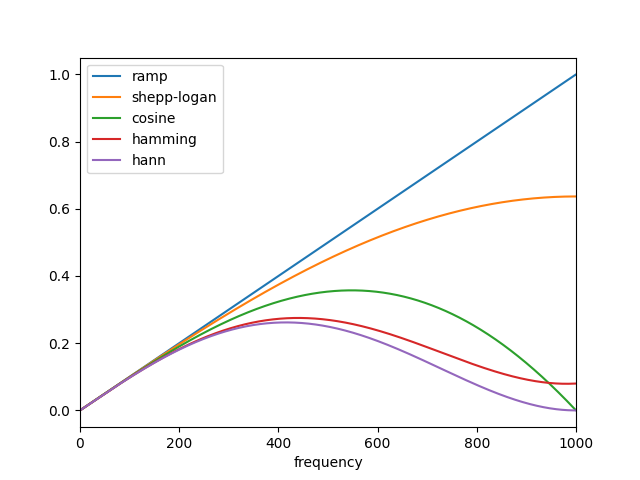
Radon transform. The only tunable parameter for the FBP is the filter,
which is applied to the Fourier transformed projections. It may be used to
suppress high frequency noise in the reconstruction. skimage provides
the filters ‘ramp’, ‘shepp-logan’, ‘cosine’, ‘hamming’, and ‘hann’:
import matplotlib.pyplot as plt
from skimage.transform.radon_transform import _get_fourier_filter

filters = ['ramp', 'shepp-logan', 'cosine', 'hamming', 'hann']

for ix, f in enumerate(filters):
    response = _get_fourier_filter(2000, f)
    plt.plot(response, label=f)

plt.xlim([0, 1000])
plt.xlabel('frequency')
plt.legend()
plt.show()
Applying the inverse radon transformation with the ‘ramp’ filter, we get:
from skimage.transform import iradon

reconstruction_fbp = iradon(sinogram, theta=theta, filter_name='ramp')
error = reconstruction_fbp - image
print(f'FBP rms reconstruction error: {np.sqrt(np.mean(error**2)):.3g}')

imkwargs = dict(vmin=-0.2, vmax=0.2)
fig, (ax1, ax2) = plt.subplots(1, 2, figsize=(8, 4.5), sharex=True, sharey=True)
ax1.set_title("Reconstruction\nFiltered back projection")
ax1.imshow(reconstruction_fbp, cmap=plt.cm.Greys_r)
ax2.set_title("Reconstruction error\nFiltered back projection")
ax2.imshow(reconstruction_fbp - image, cmap=plt.cm.Greys_r, **imkwargs)
plt.show()
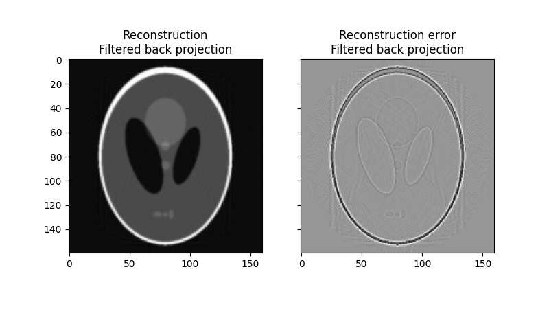
FBP rms reconstruction error: 0.0283
Reconstruction with the Simultaneous Algebraic Reconstruction Technique#
Algebraic reconstruction techniques for tomography are based on a straightforward idea: for a pixelated image the value of a single ray in a particular projection is simply a sum of all the pixels the ray passes through on its way through the object. This is a way of expressing the forward Radon transform. The inverse Radon transform can then be formulated as a (large) set of linear equations. As each ray passes through a small fraction of the pixels in the image, this set of equations is sparse, allowing iterative solvers for sparse linear systems to tackle the system of equations. One iterative method has been particularly popular, namely Kaczmarz’ method [3], which has the property that the solution will approach a least-squares solution of the equation set.
The combination of the formulation of the reconstruction problem as a set of linear equations and an iterative solver makes algebraic techniques relatively flexible, hence some forms of prior knowledge can be incorporated with relative ease.
skimage provides one of the more popular variations of the algebraic
reconstruction techniques: the Simultaneous Algebraic Reconstruction
Technique (SART) [4]. It uses Kaczmarz’ method as the iterative
solver. A good reconstruction is normally obtained in a single iteration,
making the method computationally effective. Running one or more extra
iterations will normally improve the reconstruction of sharp, high
frequency features and reduce the mean squared error at the expense of
increased high frequency noise (the user will need to decide on what number
of iterations is best suited to the problem at hand. The implementation in
skimage allows prior information of the form of a lower and upper
threshold on the reconstructed values to be supplied to the reconstruction.
from skimage.transform import iradon_sart

reconstruction_sart = iradon_sart(sinogram, theta=theta)
error = reconstruction_sart - image
print(
    f'SART (1 iteration) rms reconstruction error: ' f'{np.sqrt(np.mean(error**2)):.3g}'
)

fig, axes = plt.subplots(2, 2, figsize=(8, 8.5), sharex=True, sharey=True)
ax = axes.ravel()

ax[0].set_title("Reconstruction\nSART")
ax[0].imshow(reconstruction_sart, cmap=plt.cm.Greys_r)

ax[1].set_title("Reconstruction error\nSART")
ax[1].imshow(reconstruction_sart - image, cmap=plt.cm.Greys_r, **imkwargs)

# Run a second iteration of SART by supplying the reconstruction
# from the first iteration as an initial estimate
reconstruction_sart2 = iradon_sart(sinogram, theta=theta, image=reconstruction_sart)
error = reconstruction_sart2 - image
print(
    f'SART (2 iterations) rms reconstruction error: '
    f'{np.sqrt(np.mean(error**2)):.3g}'
)

ax[2].set_title("Reconstruction\nSART, 2 iterations")
ax[2].imshow(reconstruction_sart2, cmap=plt.cm.Greys_r)

ax[3].set_title("Reconstruction error\nSART, 2 iterations")
ax[3].imshow(reconstruction_sart2 - image, cmap=plt.cm.Greys_r, **imkwargs)
plt.show()
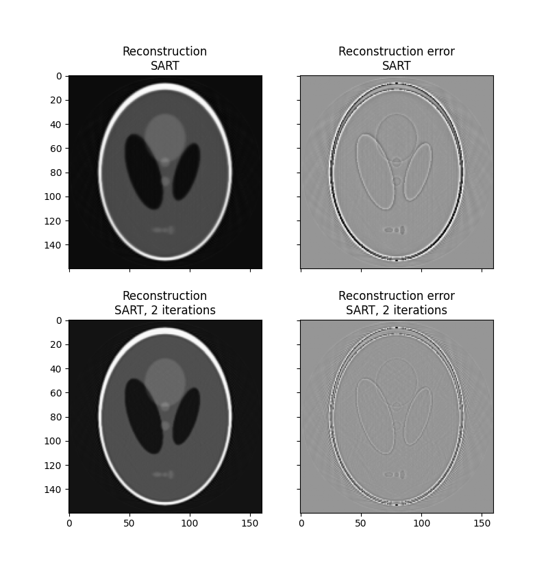
SART (1 iteration) rms reconstruction error: 0.0329
SART (2 iterations) rms reconstruction error: 0.0214
Total running time of the script: (0 minutes 1.930 seconds)