assisted-by - Unknown Directive
assisted-by - Unknown Directiveclaude-code:claude-opus-5
shape_index built its Hessian with finite differences up to scikit-image 0.26.
From 0.27 it uses the moment-corrected Gaussian derivative kernels of
hessian_matrix. on_hessian.md and hessian_review.md measure why the
Hessian changed. This notebook asks what the change does to the shape index,
and whether the old route has any claim left.
The answer is that the shape index is not the Hessian, and the ordering can
reverse: below a crossover near sigma 0.7 the finite-difference shape index is
closer to a closed form than the Gaussian-derivative one, while its Hessian is
further away.
Subscripts and name the image axes in skimage’s rc order: axis is
the first array axis, down the rows, and axis the second, across the
columns.
from itertools import combinations_with_replacement
import time

import numpy as np
import pandas as pd
import scipy.ndimage as ndi
import matplotlib.pyplot as plt
from matplotlib.colors import LinearSegmentedColormap, TwoSlopeNorm

from nbhelper import show_table
# The subject under test.
import skimage as ski
from skimage.feature import shape_index, hessian_matrix_eigvalsfatal: not a git repository (or any of the parent directories): .git
# Slots 1 and 2 of the reference categorical palette; same palette as
# `hessian_review.md`.  Validated all-pairs: CVD dE 24.7 (protan), 32.7
# (tritan), normal-vision 33.6, all checks pass on the light surface.
C_ONE, C_TWO = "#2a78d6", "#eb6834"
INK, MUTED, RULE = "#0b0b0b", "#52514e", "#dedcd5"

# Diverging: two hues with a neutral midpoint.  The shape index is signed and
# its zero means something (a saddle), so the midpoint must be neutral.
DIV = LinearSegmentedColormap.from_list("div", [C_ONE, "#f2f1ec", C_TWO])

plt.rcParams.update(
    {"figure.dpi": 110, "font.size": 9, "axes.titlesize": 9,
     "axes.titlecolor": MUTED, "figure.facecolor": "white"}
)


def bare(ax, title=None):
    """Strip an image axes down to the pixels."""
    ax.set_xticks([]); ax.set_yticks([])
    for spine in ax.spines.values():
        spine.set_visible(False)
    if title:
        ax.set_title(title)
    return ax


def recede(ax, title=None):
    """Push a plot axes' furniture into the background."""
    ax.tick_params(labelsize=8, colors=MUTED)
    for spine in ("top", "right"):
        ax.spines[spine].set_visible(False)
    for spine in ("left", "bottom"):
        ax.spines[spine].set_color(RULE)
    if title:
        ax.set_title(title)
    return ax
1. The two routes¶
Both smooth at scale sigma and take second derivatives. They differ in what
does the differentiating.
def fd_hessian(image, sigma, mode="constant", cval=0):
    """Smooth at sigma, then two central differences: the route up to 0.26."""
    smoothed = ski.filters.gaussian(image, sigma=sigma, mode=mode, cval=cval)
    gradients = np.gradient(smoothed)
    return [np.gradient(gradients[a], axis=b)
            for a, b in combinations_with_replacement(range(image.ndim), 2)]
The Gaussian-derivative route convolves once per element with a kernel whose
discrete moments have been restored. Sampling the derivative and using the taps
as they fall leaves a kernel that responds to a constant image and under-reports
curvature; imposing sum(k) == 0 and sum(k * x**2) / 2 == 1 repairs both.
def taps(sigma, order, truncate=8):
    """1-D Gaussian derivative kernel, with its discrete moments restored."""
    radius = int(truncate * sigma + 0.5)
    x = np.arange(-radius, radius + 1, dtype=float)
    smoothing = np.exp(-(x**2) / (2 * sigma**2))
    smoothing /= smoothing.sum()
    if order == 0:
        return smoothing
    if order == 1:
        kernel = smoothing * (x / sigma**2)
        return kernel / (kernel * x).sum()
    kernel = smoothing * ((x**2 - sigma**2) / sigma**4)
    kernel = kernel - kernel.sum() * smoothing
    # Below sigma of about 0.2 the line above cancels catastrophically, so the
    # residue comes out of the centre tap, before and after the x**2 scaling.
    center = len(kernel) // 2
    kernel[center] = -(kernel[:center].sum() + kernel[center + 1:].sum())
    kernel /= (kernel * x**2).sum() / 2
    kernel[center] = -(kernel[:center].sum() + kernel[center + 1:].sum())
    return kernel


def gd_hessian(image, sigma, mode="constant", cval=0, truncate=8):
    """One separable pass per element, with the corrected kernels: 0.27 on."""
    image = np.asarray(image, dtype=float)
    ndim = image.ndim
    kernels = {(axis, o): taps(sigma, o, truncate)
               for axis in range(ndim) for o in (0, 1, 2)}
    elements = []
    for ax0, ax1 in combinations_with_replacement(range(ndim), 2):
        orders = [0] * ndim
        orders[ax0] += 1
        orders[ax1] += 1
        result = image
        for axis, o in enumerate(orders):
            result = ndi.correlate1d(result, kernels[(axis, o)], axis=axis,
                                     mode=mode, cval=cval)
        elements.append(result)
    return elements


ROUTES = (("finite differences", fd_hessian), ("Gaussian derivatives", gd_hessian))
The shape index itself is the same arithmetic either way: Koenderink and van Doorn’s measure of local curvature, built from the two Hessian eigenvalues.
def s_from(H):
    """The shape index, from upper-diagonal Hessian elements."""
    l1, l2 = hessian_matrix_eigvals(H)
    with np.errstate(divide="ignore", invalid="ignore"):
        return (2.0 / np.pi) * np.arctan((l2 + l1) / (l2 - l1))


PHOTO = ski.util.img_as_float(ski.data.camera())[::2, ::2]
The finite-difference transcription has to be the library’s, or nothing below means anything.
show_table(pd.DataFrame(
    [{"sigma": sigma,
      "transcription vs skimage.feature.shape_index":
          "bit-identical" if np.array_equal(
              np.nan_to_num(shape_index(PHOTO, sigma=sigma), nan=-9),
              np.nan_to_num(s_from(fd_hessian(PHOTO, sigma)), nan=-9))
          else "DIFFERS"}
for sigma in (0.5, 1.0, 2.0, 4.0)]), index="sigma")The Gaussian-derivative kernels are pinned by their two moment conditions, so check those instead.
def moments(sigma):
    """The two conditions that pin the second-derivative kernel."""
    k = taps(sigma, 2)
    radius = len(k) // 2
    x = np.arange(-radius, radius + 1, dtype=float)
    return {"sigma": sigma, "taps": len(k),
            "sum(k), want 0": f"{k.sum():.1e}",
            "sum(k * x**2) / 2, want 1": f"{(k * x**2).sum() / 2:.12f}"}


show_table(pd.DataFrame([moments(s) for s in (0.3, 0.5, 1.0, 2.0)]), index="sigma")2. The shape index only sees a ratio¶
The Hessian comparisons in hessian_review.md are about magnitudes. The shape
index is not: it is a function of the quotient of the two eigenvalues, so
multiplying the whole Hessian by any positive constant leaves it alone.
rng = np.random.default_rng(0)
random_H = [rng.normal(size=(64, 64)) for _ in range(3)]
baseline = s_from(random_H)

show_table(pd.DataFrame(
    [{"H scaled by": f"{c:g}",
      "max |change in s|":
          f"{np.nanmax(np.abs(s_from([c * h for h in random_H]) - baseline)):.1e}"}
for c in (0.5, 2.0, 1e3, 1e-3)]), index="H scaled by")That is the design, not an accident of the formula. Koenderink and van Doorn build the shape index from a polar coordinate system in the plane, in which “the direction encodes the shape, whereas the distance from the origin encodes the size” Koenderink & Doorn, 1992. Their definition, with , is the one the library implements:
and they note that is directly proportional to the angle with the axis. Proportional, not merely monotonic, so an error in that angle is an error in scaled by a constant.
rough = [a + 0.01 * rng.normal(size=a.shape) for a in random_H]
pair_a, pair_b = hessian_matrix_eigvals(random_H), hessian_matrix_eigvals(rough)
turn = np.arctan2(pair_b[1], pair_b[0]) - np.arctan2(pair_a[1], pair_a[0])
turn = np.abs(np.arctan2(np.sin(turn), np.cos(turn)))
moved = np.abs(s_from(rough) - s_from(random_H))
usable = np.isfinite(moved) & np.isfinite(turn) & (moved < 1.9)

show_table(pd.DataFrame([{
    "pixels compared": int(usable.sum()),
    "max |change in s - (2/pi) * change in angle|":
        f"{np.nanmax(np.abs(moved[usable] - (2 / np.pi) * turn[usable])):.1e}"}]),
index="pixels compared")So the angle is not a proxy for the shape index. It is the shape index, to a factor of . §6 uses that to take the error apart.
The companion measure in the same paper is the curvedness,
, which carries the distance from the
origin. Between them and hold everything the Hessian has. The shape
index discards entirely, and is what the moment correction of
hessian_matrix repairs.
3. How much the pictures move¶
The docstring sorts the shape index into nine named classes, from spherical cup at -1 to spherical cap at +1. The fraction of pixels that change class is the change a caller sees.
BINS = np.array([-7/8, -5/8, -3/8, -1/8, 1/8, 3/8, 5/8, 7/8])


def interior(sigma, ndim=2, truncate=8):
    """The pixels no kernel tap reached over the border."""
    reach = int(truncate * sigma + 0.5) + 1
    return (slice(reach, -reach),) * ndim


def change_row(image, sigma):
    """How far the two routes disagree on one image at one scale."""
    inner = interior(sigma)
    a = s_from(fd_hessian(image, sigma))[inner]
    b = s_from(gd_hessian(image, sigma))[inner]
    ok = ~np.isnan(a) & ~np.isnan(b)
    return {"sigma": sigma,
            "pixels changing class":
                f"{100 * np.mean(np.digitize(a[ok], BINS) != np.digitize(b[ok], BINS)):.1f}%",
            "median |change in s|": f"{np.median(np.abs(a[ok] - b[ok])):.3f}",
            "NaN, FD": int(np.isnan(a).sum()), "NaN, GD": int(np.isnan(b).sum())}


show_table(pd.DataFrame([change_row(PHOTO, s) for s in (0.5, 1.0, 2.0, 4.0)]),
index="sigma")At sigma of 0.5 most of the picture is reclassified; by sigma of 4 almost
none of it is. Neither route produces NaN on this photograph, so the undefined
flat regions the docstring warns about do not arise here.
fig, axes = plt.subplots(1, 3, figsize=(8.4, 3.0))
VIEW_SIGMA = 1.0
inner = interior(VIEW_SIGMA)
sfd = s_from(fd_hessian(PHOTO, VIEW_SIGMA))[inner]
sgd = s_from(gd_hessian(PHOTO, VIEW_SIGMA))[inner]

for ax, data, title in ((axes[0], sfd, "finite differences"),
                        (axes[1], sgd, "Gaussian derivatives")):
    bare(ax, title).imshow(data, cmap=DIV, norm=TwoSlopeNorm(0, -1, 1))
limit = np.abs(sgd - sfd).max()
third = bare(axes[2], "difference").imshow(
    sgd - sfd, cmap=DIV, norm=TwoSlopeNorm(0, -limit, limit))
fig.colorbar(third, ax=axes[2], fraction=0.046).outline.set_visible(False)
fig.suptitle(f"shape index on camera at sigma = {VIEW_SIGMA}, cup (blue) to cap (orange)",
             color=MUTED, fontsize=9)
fig.tight_layout()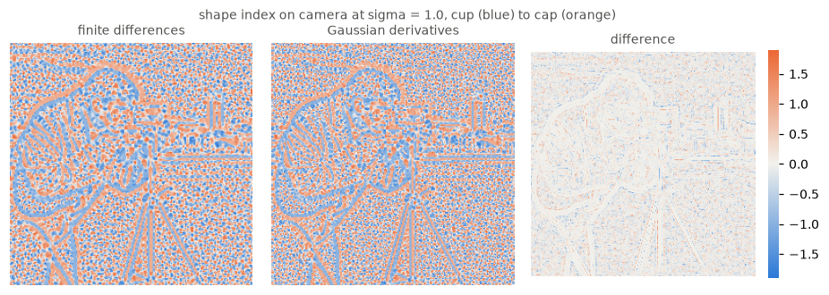
The difference is structured rather than scattered. Splitting the frame by how far the eigenvalue pair is from isotropic shows where it concentrates.
pair = hessian_matrix_eigvals(gd_hessian(PHOTO, VIEW_SIGMA))
with np.errstate(divide="ignore", invalid="ignore"):
    anisotropy = (np.abs(pair[0] - pair[1])
                  / np.maximum(np.abs(pair[0]), np.abs(pair[1])))[inner]
gap = np.abs(sgd - sfd)
usable = np.isfinite(gap) & np.isfinite(anisotropy)
edges = np.nanpercentile(anisotropy[usable], [0, 20, 40, 60, 80, 100])

show_table(pd.DataFrame(
    [{"|l1 - l2| / max|l|": f"{edges[k]:.2f} to {edges[k+1]:.2f}",
      "median |change in s|":
          f"{np.median(gap[usable & (anisotropy >= edges[k]) & (anisotropy <= edges[k+1])]):.4f}"}
for k in range(5)]), index="|l1 - l2| / max|l|")The disagreement is smallest in the middle of that range and largest at the top, where the two eigenvalues approach equal and opposite, which is where the saddles are. The rank correlation over the individual pixels is only +0.21, so this is a tendency rather than a rule, and the figure is the better description of the pattern.
4. Which one is right¶
A Gaussian blob smoothed by a Gaussian is a Gaussian, so its Hessian and therefore its shape index are known in closed form. That makes a standard neither route was built against.
def blob_truth(size, width, sigma):
    """A Gaussian blob, and the exact shape index of its smoothing."""
    r, c = [x - size // 2 for x in np.indices((size, size), dtype=float)]
    image = np.exp(-(r**2 + c**2) / (2 * width**2))
    spread = width**2 + sigma**2
    amp = (width**2 / spread) * np.exp(-(r**2 + c**2) / (2 * spread))
    H = [amp * (r**2 - spread) / spread**2,
         amp * (r * c) / spread**2,
         amp * (c**2 - spread) / spread**2]
    return image, H


SIGMAS = (0.3, 0.5, 0.8, 1.0, 1.5, 2.0, 4.0)
BLOB_SIZE, BLOB_WIDTH = 201, 6.0


def blob_error(route, sigma):
    """Mean |s - s_exact| over the interior of the blob."""
    image, H_true = blob_truth(BLOB_SIZE, BLOB_WIDTH, sigma)
    inner = interior(sigma)
    truth = s_from(H_true)
    return np.nanmean(np.abs(s_from(route(image, sigma))[inner] - truth[inner]))


errors = {name: [blob_error(route, s) for s in SIGMAS] for name, route in ROUTES}
show_table(pd.DataFrame(
    [{"sigma": s,
      **{name: f"{errors[name][k]:.2e}" for name, _ in ROUTES},
      "closer": min(ROUTES, key=lambda nr: errors[nr[0]][k])[0],
      "by": f"{max(errors[n][k] for n, _ in ROUTES) / min(errors[n][k] for n, _ in ROUTES):.0f}x"}
for k, s in enumerate(SIGMAS)]), index="sigma")The ordering reverses between sigma 0.5 and 0.8 on this grid; §10 sweeps
finely and puts the crossover at 0.70 for this blob. Below it the
finite-difference shape index is the closer of the two, by a factor of 14 at
sigma 0.5 and 28 at sigma 0.3. Above it the Gaussian-derivative one wins,
and by four orders of magnitude by sigma 2.
fig, ax = plt.subplots(figsize=(5.6, 3.2))
for (name, _), colour in zip(ROUTES, (C_TWO, C_ONE)):
    ax.semilogy(SIGMAS, errors[name], "-o", color=colour, linewidth=2,
                markersize=6, label=name)
ax.axvline(0.70, color=RULE, linewidth=1, zorder=0)   # located in section 10
ax.annotate("crossover, 0.70", (0.68, 3e-7), color=MUTED, fontsize=8,
            rotation=90, va="bottom", ha="right")
ax.set_xticks(SIGMAS)
ax.set_xticklabels([str(s) for s in SIGMAS])
recede(ax, "mean |s - s_exact| on a smoothed Gaussian blob")
ax.set_xlabel("sigma", color=MUTED)
ax.legend(frameon=False, fontsize=8, labelcolor=MUTED)
fig.tight_layout()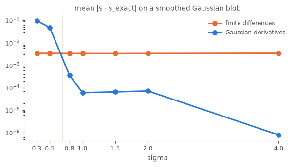
5. A better Hessian, a worse shape index¶
The reversal is not the Gaussian-derivative Hessian being worse at small
sigma. On the same images it is better at every scale measured.
def hessian_error(route, sigma):
    """Worst element error over the interior, as a fraction of the peak."""
    image, H_true = blob_truth(BLOB_SIZE, BLOB_WIDTH, sigma)
    inner = interior(sigma)
    peak = max(np.abs(h[inner]).max() for h in H_true)
    return max(np.abs(a[inner] - b[inner]).max()
               for a, b in zip(route(image, sigma), H_true)) / peak


show_table(pd.DataFrame(
    [{"sigma": s,
      **{f"H, {name}": f"{hessian_error(route, s):.2e}" for name, route in ROUTES},
      "H closer": min(ROUTES, key=lambda nr: hessian_error(nr[1], s))[0],
      "s closer": min(ROUTES, key=lambda nr: errors[nr[0]][k])[0]}
for k, s in enumerate((0.3, 0.5, 0.8, 1.0, 2.0))]), index="sigma")At sigma 0.3 and 0.5 the Gaussian-derivative Hessian is the closer one and its
shape index is the further one. The accuracy of a Hessian is therefore not a
proxy for the accuracy of the shape index built from it, and §2 is why: the
shape index discards exactly the part of the Hessian that the moment correction
repairs.
6. What turns the eigenvalue pair¶
§2 showed the angle of the eigenvalue pair is the shape index, to a factor of . Measuring the angle is therefore not a different experiment from §4; it is the same error, in units that can be taken apart element by element.
def angle_error(H, H_true, inner):
    """Median angular error of the eigenvalue pair, in radians."""
    lt = hessian_matrix_eigvals(H_true)
    lc = hessian_matrix_eigvals(H)
    at = np.arctan2(lt[1][inner], lt[0][inner])
    ac = np.arctan2(lc[1][inner], lc[0][inner])
    return np.median(np.abs(np.arctan2(np.sin(ac - at), np.cos(ac - at))))


def angle_row(sigma):
    """Angular error of each route at one scale."""
    image, H_true = blob_truth(BLOB_SIZE, BLOB_WIDTH, sigma)
    inner = interior(sigma)
    return {"sigma": sigma,
            **{name: f"{angle_error(route(image, sigma), H_true, inner):.2e}"
               for name, route in ROUTES}}


show_table(pd.DataFrame([angle_row(s) for s in (0.3, 0.5, 1.0, 2.0)]),
index="sigma")The finite-difference angular error is flat at about radians
at every scale, because its stencil error is set by the pixel grid and not by
sigma. The Gaussian-derivative one starts an order of magnitude worse and
falls away to nothing.
Which element carries it is decidable: substitute the exact value for one element and measure the angle again.
def swap_rows(sigma):
    """Angular error with each element in turn replaced by its exact value."""
    image, H_true = blob_truth(BLOB_SIZE, BLOB_WIDTH, sigma)
    inner = interior(sigma)
    out = []
    for name, route in ROUTES:
        H = route(image, sigma)
        out.append({
            "sigma": sigma, "route": name,
            "as computed": f"{angle_error(H, H_true, inner):.2e}",
            "exact mixed element":
                f"{angle_error([H[0], H_true[1], H[2]], H_true, inner):.2e}",
            "exact diagonals":
                f"{angle_error([H_true[0], H[1], H_true[2]], H_true, inner):.2e}"})
    return out


show_table(pd.DataFrame([r for s in (0.3, 0.5, 1.0) for r in swap_rows(s)]),
index="sigma")Two different stories in one table.
For the Gaussian-derivative route at sigma 0.3, handing it the exact mixed
element drops the angular error by a factor of about 50, and handing it the
exact diagonals does not help at all (0.119 against 0.108 as computed). Its
small-sigma shape-index error is the mixed
element. That follows from how the kernels are built: the diagonal elements get
the second-derivative kernel, whose moment correction forces exactness on a
quadratic, while the mixed element is two first-derivative kernels whose
correction fixes only the first moment.
For the finite-difference route, handing it the exact mixed element makes the angle nine times worse, and the exact diagonals twenty-seven times worse. Its small angular error is not accuracy in any element. It is three element errors that cancel, and repairing any one of them destroys the cancellation.
7. Reasons to prefer the finite-difference result¶
Three were measurable. The first is §4’s accuracy below the crossover. The second is noise.
def noise_row(sigma, amplitude, draws=12):
    """Spread of s under repeated noise, where the blob has real curvature."""
    image, _ = blob_truth(BLOB_SIZE, BLOB_WIDTH, 1.0)
    _, H_true = blob_truth(BLOB_SIZE, BLOB_WIDTH, sigma)
    strength = np.sqrt(H_true[0]**2 + 2 * H_true[1]**2 + H_true[2]**2)
    inner = interior(sigma)
    mask = (strength > 0.3 * strength.max())[inner]
    rng = np.random.default_rng(0)
    draws_by_route = {name: [] for name, _ in ROUTES}
    for _ in range(draws):
        noisy = image + amplitude * rng.normal(size=image.shape)
        for name, route in ROUTES:
            draws_by_route[name].append(s_from(route(noisy, sigma))[inner])
    row = {"sigma": sigma, "noise": amplitude}
    for name, _ in ROUTES:
        stack = np.stack(draws_by_route[name])
        row[name] = f"{np.nanmean(np.nanstd(stack, axis=0)[mask]):.4f}"
    return row


show_table(pd.DataFrame([noise_row(s, a) for s in (1.0, 2.0)
for a in (0.005, 0.02)]), index="sigma")The finite-difference shape index is the steadier of the two under noise, by
about 1.8 times at sigma 1 and 1.2 times at sigma 2. Its stencil spans two
pixels rather than one and rolls off towards Nyquist, so it passes less of the
noise that a second derivative amplifies.
The third is cost.
rows = []
for sigma in (0.5, 1.0, 2.0, 4.0):
    timing = {}
    for name, route in ROUTES:
        runs = []
        for _ in range(3):                      # best of three, not the mean
            started = time.perf_counter()
            route(PHOTO, sigma)
            runs.append(time.perf_counter() - started)
        timing[name] = min(runs)
    rows.append({"sigma": sigma,
                 **{n: f"{t * 1e3:.1f} ms" for n, t in timing.items()},
                 "ratio": f"{timing[ROUTES[1][0]] / timing[ROUTES[0][0]]:.1f}x"})
show_table(pd.DataFrame(rows), index="sigma")The corrected kernels are truncated at eight standard deviations, so they grow
with sigma where the central differences do not.
The fourth reason is not measurable here and is the strongest: a published
result computed with the old route is reproduced only by the old route.
skimage2.migration.shape_index_finite_difference is that route, kept for the
purpose.
8. What other libraries do¶
The shape index is implemented elsewhere, but almost entirely on explicit
surfaces -- triangle meshes or fields of normals -- rather than on a raster.
FreeSurfer’s mris_curvature_stats, pycurv, VCGLib and the eos library all
carry it; MIRTK carries the curvedness without it. ITK, SimpleITK, VIGRA,
DIPlib, OpenCV and Pillow carry neither.
That matters for §4 and §7: a mesh implementation fits a quadratic to a vertex neighbourhood, so it never has to choose between finite differences and Gaussian derivatives. The choice this notebook is about belongs to the raster setting, and there is no other library in that setting to check against.
The implementations that do exist disagree with each other on two things. The first is the sign.
from math import atan, pi

DOME = (-1.0, -2.0)            # k1 >= k2, both negative: a dome


def library_forms(k1, k2):
    """The same dome, under each library's published expression."""
    return [
        {"library": "scikit-image, after Koenderink",
         "expression": "(2/pi) atan((k2+k1)/(k2-k1))",
         "s": f"{2 / pi * atan((k2 + k1) / (k2 - k1)):+.3f}"},
        {"library": "pycurv",
         "expression": "(2/pi) atan((k1+k2)/(k1-k2))",
         "s": f"{2 / pi * atan((k1 + k2) / (k1 - k2)):+.3f}"},
        {"library": "FreeSurfer",
         "expression": "atan((k1+k2)/(k2-k1))",
         "s": f"{atan((k1 + k2) / (k2 - k1)):+.3f}"},
    ]


show_table(pd.DataFrame(library_forms(*DOME)), index="library")pycurv reverses the denominator, so its shape index is the negative of
Koenderink’s: the dome that scikit-image scores at +0.795 it scores at
-0.795. FreeSurfer omits the , so its range is
rather than . scikit-image follows the paper exactly, in the formula,
in the ordering, and in the nine category bounds of
the docstring table.
The second disagreement is the degenerate case, and it is the subject of §9. FreeSurfer returns 0 when the two curvatures are equal:
return (af_k1 == af_k2 ? 0 : atan((af_k1+af_k2)/(af_k2 - af_k1)));pycurv returns 0 only when both are zero, and leaves the equal-and-non-zero
case to the arithmetic:
if kappa_1 == 0 and kappa_2 == 0:
    return 0
else:
    return 2 / pi * atan((kappa_1 + kappa_2) / (kappa_1 - kappa_2))
Neither matches the paper. §9 is what the paper asks for.
FreeSurfer puts the shape index behind an explicit --shapeIndex command-line
flag, with the comment “The ‘Shape Index’ can be problematic due to the atan
calculations”, so the fragility §9 measures has been met before.
9. What not to conclude¶
9.1 The accuracy below the crossover is not a property to rely on¶
§6 is the reason. The finite-difference route is close on the angle because its three element errors cancel, not because any element is right. Whether the cancellation holds for an image unlike this blob is not measured here, and it cannot be with the method used: §4 needs a closed form, which a photograph does not have. A property that survives only while three errors stay in step is a coincidence to be grateful for, not a design to depend on.
10. Should the library switch route below the crossover¶
§4 found the finite-difference shape index closer to the closed form at small
sigma, so the question is whether shape_index should dispatch on sigma.
Three measurements say no.
The first is that the crossover is a property of the image, not a constant.
def crossover(width, size=201, grid=np.arange(0.3, 2.01, 0.05)):
    """The smallest sigma at which Gaussian derivatives overtake."""
    for sigma in grid:
        image, H_true = blob_truth(size, width, sigma)
        inner = interior(sigma)
        truth = s_from(H_true)
        errs = [np.nanmean(np.abs(s_from(route(image, sigma))[inner] - truth[inner]))
                for _, route in ROUTES]
        if errs[1] < errs[0]:
            return sigma
    return np.nan


show_table(pd.DataFrame(
    [{"blob width": w, "size": 201 if w <= 10 else 301,
      "crossover sigma": f"{crossover(w, 201 if w <= 10 else 301):.2f}"}
for w in (2.0, 3.0, 6.0, 10.0, 16.0)]), index="blob width")It moves between 0.55 and 0.70 over blob widths from 2 to 16 pixels, on the one
family of shapes where a closed form exists at all. A photograph contains many
widths at once, so no single sigma divides the two regimes for a whole image.
The second is that a switch is a discontinuity in sigma, and the shape index
is often swept over sigma.
def step(low, high):
    """What a reader sees across a sigma step, switching or not."""
    inner = interior(high)
    before = s_from(fd_hessian(PHOTO, low))[inner]
    after = s_from(gd_hessian(PHOTO, high))[inner]
    unswitched = s_from(gd_hessian(PHOTO, low))[inner]
    ok = np.isfinite(before) & np.isfinite(after) & np.isfinite(unswitched)
    return {"sigma step": f"{low} to {high}",
            "median |ds|, switching route": f"{np.median(np.abs(after - before)[ok]):.3f}",
            "median |ds|, staying on one": f"{np.median(np.abs(after - unswitched)[ok]):.3f}"}


show_table(pd.DataFrame([step(0.79, 0.81), step(0.75, 0.85)]), index="sigma step")Across a sigma step of 0.02 a switch moves the shape index by 0.134, where
staying on one route moves it by 0.011. The artefact is twelve times the signal,
and more than half the width of a category bin from the docstring table.
The third is §6. The advantage being bought is a cancellation of three element
errors, and §6 locates the Gaussian-derivative shortfall in the mixed element.
A better mixed-element kernel is worth having on its own account, but it does
not remove the reason for a switch: imposing the first-derivative kernel’s third
moment, which is 270% out at sigma 0.3 and exact above 0.8, improves the mixed
element by about 50 times and the typical shape-index pixel by 3 to 6 times, and
still moves the crossover only from 0.70 to 0.65. The gap below the crossover is
not the mixed element alone.
Callers who want the old numbers at every sigma, continuously, already have
them in skimage2.migration.shape_index_finite_difference.
11. The umbilic, where the formula cannot say what the paper says¶
Koenderink and van Doorn separate two degenerate cases, and only one of them is undefined Koenderink & Doorn, 1992. At a planar point, , the direction in the plane is the direction of the origin, so the shape index “is really indeterminate”, as they put it, and NaN is the right answer. At an umbilic, , it is not indeterminate: it is for the outside of a sphere and for the inside, and those are “true endpoints of the scale”.
The formula cannot deliver that. It reads the sign of , which at an umbilic is zero, so the answer comes from a rounding residue.
image, H_true = blob_truth(BLOB_SIZE, BLOB_WIDTH, 0.5)
middle = BLOB_SIZE // 2
rows = []
for name, H in (("exact", H_true), ("finite differences", fd_hessian(image, 0.5)),
                ("Gaussian derivatives", gd_hessian(image, 0.5))):
    l1, l2 = hessian_matrix_eigvals(H)
    a, b = l1[middle, middle], l2[middle, middle]
    with np.errstate(divide="ignore", invalid="ignore"):
        rows.append({"route": name, "lambda1": f"{a:.6e}", "lambda2": f"{b:.6e}",
                     "lambda2 - lambda1": f"{b - a:.1e}",
                     "s": f"{(2 / np.pi) * np.arctan((b + a) / (b - a)):+.4f}"})
show_table(pd.DataFrame(rows), index="route")At the centre of a radially symmetric blob the two curvatures are equal, so
lambda2 - lambda1 is either exactly zero or a residue of order 10-17, and
its sign sends the shape index to -1 or +1 — spherical cup or spherical cap,
the two ends of the scale. This is a determinate value that the implementation
cannot reach, not a quantity the two routes disagree about on their merits.
The two computed routes do at least agree with each other, and flip together with the sign of the curvature. The exact Hessian, whose residue is a positive zero rather than a negative one, lands on the other end in both cases.
def umbilic_row(label, image, name, H):
    """The shape index at the centre, where the two curvatures are equal."""
    l1, l2 = hessian_matrix_eigvals(H)
    middle = BLOB_SIZE // 2
    a, b = l1[middle, middle], l2[middle, middle]
    with np.errstate(divide="ignore", invalid="ignore"):
        return {"blob": label, "route": name, "k1 = k2": f"{a:+.3e}",
                "k2 - k1": f"{b - a:+.1e}",
                "s": f"{(2 / np.pi) * np.arctan((b + a) / (b - a)):+.1f}"}


bright, H_bright = blob_truth(BLOB_SIZE, BLOB_WIDTH, 1.0)
rows = []
for label, image, H_exact in (("bright (local max)", bright, H_bright),
                              ("dark (local min)", -bright,
                               [-h for h in H_bright])):
    rows.append(umbilic_row(label, image, "exact", H_exact))
    for name, route in ROUTES:
        rows.append(umbilic_row(label, image, name, route(image, 1.0)))
show_table(pd.DataFrame(rows), index="blob")It needs near-exact symmetry, so it is a synthetic-image problem:
def near_isotropic(H):
    """Pixels where |l1 - l2| is within rounding of zero."""
    l1, l2 = hessian_matrix_eigvals(H)
    scale = np.maximum(np.abs(l1), np.abs(l2))
    with np.errstate(divide="ignore", invalid="ignore"):
        return np.nansum(np.abs(l1 - l2) / scale < 1e-12)


blob, _ = blob_truth(BLOB_SIZE, BLOB_WIDTH, 1.0)
show_table(pd.DataFrame(
    [{"image": label, "pixels": image.size,
      **{name: int(near_isotropic(route(image, 1.0))) for name, route in ROUTES}}
     for label, image in (("camera, 256x256", PHOTO),
("Gaussian blob, 201x201", blob))]), index="image")12. A more careful mixed element¶
§6 put the Gaussian-derivative shortfall in the mixed element. That element is two passes of the first-derivative kernel, so the question is which of its moments is wrong.
correlate1d at the origin returns sum(k * x**n) for . Smoothing
at scale gives , whose derivative at the
origin is . So the kernel owes three conditions, and the shipped one
imposes the first two.
def first_moments(sigma):
    """What the shipped first-derivative kernel gets right and wrong."""
    k = taps(sigma, 1)
    radius = len(k) // 2
    x = np.arange(-radius, radius + 1, dtype=float)
    third, want = (k * x**3).sum(), 3 * sigma**2
    return {"sigma": sigma, "taps": len(k),
            "sum(k), want 0": f"{k.sum():.0e}",
            "sum(k * x), want 1": f"{(k * x).sum():.6f}",
            "sum(k * x**3)": f"{third:.4f}",
            "want 3 sigma**2": f"{want:.4f}",
            "relative error": f"{abs(third - want) / want:.1%}"}


show_table(pd.DataFrame([first_moments(s) for s in (0.3, 0.5, 0.8, 1.0, 2.0)]),
index="sigma")The third moment is 270% out at sigma 0.3 and exact from about 0.8, which is
where the crossover of §10 sits. Below sigma of about 0.5 the kernel has
collapsed towards the plain central difference ,
whose third moment is 1 whatever sigma is, while the truth asks for
.
Imposing it needs one more degree of freedom. Two odd basis functions carry two conditions.
def taps1_third(sigma, truncate=8):
    """First-derivative kernel with the first and third moments imposed."""
    radius = int(truncate * sigma + 0.5)
    x = np.arange(-radius, radius + 1, dtype=float)
    g = np.exp(-(x**2) / (2 * sigma**2))
    g /= g.sum()
    basis = (g * (x / sigma**2), g * (x**3 / sigma**4))
    M = np.array([[(b * x).sum() for b in basis],
                  [(b * x**3).sum() for b in basis]])
    weights = np.linalg.solve(M, np.array([1.0, 3.0 * sigma**2]))
    return weights[0] * basis[0] + weights[1] * basis[1], np.linalg.cond(M)


show_table(pd.DataFrame(
    [{"sigma": s, "cond(M)": f"{taps1_third(s)[1]:.1e}",
      "sum(k * x)": f"{(taps1_third(s)[0] * np.arange(-(len(taps1_third(s)[0]) // 2), len(taps1_third(s)[0]) // 2 + 1)).sum():.6f}",
      "largest change vs shipped": f"{np.abs(taps1_third(s)[0] - taps(s, 1)).max():.3f}"}
for s in (0.3, 0.5, 0.8, 1.0, 2.0)]), index="sigma")The change is 0.12 of a tap at sigma 0.3, 3e-4 at 0.8 and nothing at 1.0, so
it cannot disturb the regime that already works. The 2 by 2 system is badly
conditioned at sigma 0.3, which is the first thing to watch.
def gd_third(image, sigma, mode="constant", cval=0, truncate=8):
    """gd_hessian with the third moment imposed on the first derivative."""
    image = np.asarray(image, dtype=float)
    ndim = image.ndim
    kernels = {0: taps(sigma, 0, truncate), 1: taps1_third(sigma, truncate)[0],
               2: taps(sigma, 2, truncate)}
    elements = []
    for ax0, ax1 in combinations_with_replacement(range(ndim), 2):
        orders = [0] * ndim
        orders[ax0] += 1
        orders[ax1] += 1
        result = image
        for axis, o in enumerate(orders):
            result = ndi.correlate1d(result, kernels[o], axis=axis,
                                     mode=mode, cval=cval)
        elements.append(result)
    return elements


def mixed_row(sigma):
    """Mixed element, angle, and shape index, for the three kernels."""
    image, H_true = blob_truth(BLOB_SIZE, BLOB_WIDTH, sigma)
    inner = interior(sigma)
    peak = max(np.abs(h[inner]).max() for h in H_true)
    truth = s_from(H_true)
    row = {"sigma": sigma}
    for name, H in (("shipped", gd_hessian(image, sigma)),
                    ("third moment", gd_third(image, sigma))):
        row[f"Hij, {name}"] = f"{np.abs(H[1][inner] - H_true[1][inner]).max() / peak:.1e}"
        row[f"angle, {name}"] = f"{angle_error(H, H_true, inner):.1e}"
        row[f"median |ds|, {name}"] = \
            f"{np.nanmedian(np.abs(s_from(H)[inner] - truth[inner])):.1e}"
    row["median |ds|, FD"] = \
        f"{np.nanmedian(np.abs(s_from(fd_hessian(image, sigma))[inner] - truth[inner])):.1e}"
    return row


show_table(pd.DataFrame([mixed_row(s) for s in (0.3, 0.5, 0.8, 1.0)]), index="sigma")The mixed element improves by about fifty times at the small scales where it was wrong, and by less as the shipped kernel comes right. The typical shape-index pixel improves by three to six times, which is what §2 says it must: the angle and the shape index move together, and they do.
It still does not reach the finite-difference route, and the crossover barely moves.
def crossover_for(route, grid=np.arange(0.3, 1.21, 0.05)):
    """The smallest sigma at which `route` overtakes finite differences."""
    for sigma in grid:
        image, H_true = blob_truth(BLOB_SIZE, BLOB_WIDTH, sigma)
        inner = interior(sigma)
        truth = s_from(H_true)
        fd = np.nanmean(np.abs(s_from(fd_hessian(image, sigma))[inner] - truth[inner]))
        gd = np.nanmean(np.abs(s_from(route(image, sigma))[inner] - truth[inner]))
        if gd < fd:
            return sigma
    return np.nan


show_table(pd.DataFrame(
    [{"kernel": name, "crossover sigma": f"{crossover_for(route):.2f}"}
     for name, route in (("shipped", gd_hessian), ("third moment", gd_third))]),
index="kernel")So the correction is worth having on its own account — a fifty times better
mixed element at small sigma, negligible above 0.8, one more condition on a
kernel that already carries two — and it is not an answer to §10. The gap below the
crossover is not the mixed element alone.
12.1 The blob flatters finite differences¶
§4 measures against a Gaussian blob because that is the only shape with a closed form. A blob is also the input least able to show what finite differences get wrong, because a central difference errs on high spatial frequencies and a smoothed blob has almost none.
def fd_cost(image, sigma, truth=None):
    """FD's error, and how often it changes the category."""
    inner = interior(sigma)
    a = s_from(fd_hessian(image, sigma))[inner]
    b = (s_from(gd_hessian(image, sigma))[inner] if truth is None
         else s_from(truth)[inner])
    ok = np.isfinite(a) & np.isfinite(b)
    return (f"{np.median(np.abs(a - b)[ok]):.4f}",
            f"{100 * np.mean(np.digitize(a[ok], BINS) != np.digitize(b[ok], BINS)):.2f}%")


rows = []
for sigma in (2.0, 4.0, 8.0):
    blob_image, blob_H = blob_truth(401, 12.0, sigma)
    med_b, cls_b = fd_cost(blob_image, sigma, truth=blob_H)
    med_p, cls_p = fd_cost(PHOTO, sigma)
    rows.append({"sigma": sigma, "blob, median |ds|": med_b, "blob, wrong class": cls_b,
                 "camera, median |ds|": med_p, "camera, wrong class": cls_p})
show_table(pd.DataFrame(rows), index="sigma")At sigma 2 the finite-difference error is twenty times larger on the
photograph than on the blob, and it moves 16% of pixels across a category
boundary against 0.03%. It decays as sigma removes the frequencies the stencil
gets wrong, and by sigma 8 it is under 1% on both.
Part of that gap is that a photograph has more pixels sitting near a boundary, but only a small part.
def boundary_distance(image, sigma):
    """Median distance from the shape index to the nearest category edge."""
    inner = interior(sigma)
    s = s_from(gd_hessian(image, sigma))[inner]
    s = s[np.isfinite(s)]
    return np.median(np.min(np.abs(s[..., None] - BINS), axis=-1))


blob_image, _ = blob_truth(401, 12.0, 2.0)
show_table(pd.DataFrame(
    [{"image": label, "median distance to a category edge":
      f"{boundary_distance(image, 2.0):.4f}"}
     for label, image in (("camera", PHOTO), ("Gaussian blob", blob_image))]),
index="image")A factor of 1.8 in boundary proximity against a factor of 20 in the error, so most of the difference is the error itself and not the binning. Read §4’s numbers as the best case for finite differences, not the typical one.
13. Summary¶
| question | answer |
|---|---|
| how much does the shape index move | 71% of pixels change class at sigma 0.5, 46% at 1, 16% at 2, 5% at 4 |
| which is closer to a closed form | finite differences below the crossover, Gaussian derivatives above, by up to |
| where the crossover is | sigma 0.70 for a blob of width 6; 0.55 to 0.70 over widths 2 to 16 |
| is the better Hessian the better shape index | no: at sigma 0.3 and 0.5 the Gaussian-derivative Hessian is closer and its shape index is further |
| why | the shape index sees only the eigenvalue pair’s angle; the Gaussian-derivative angle error is all in the mixed element, and the finite-difference one is three errors cancelling |
| reasons to keep the old route | accuracy below the crossover; 1.2 to 1.8 times steadier under noise; cheaper, and more so as sigma grows; bit-reproducibility of published numbers |
should the library switch route at small sigma | no: the crossover moves with the image, and a switch jumps s by 0.134 against a real change of 0.011 |
| does a better mixed element close the gap | no: the third moment improves the mixed element 50x and the typical pixel 3-6x, and moves the crossover only 0.70 to 0.65 |
is the FD error important at large sigma | on a photograph yes up to sigma about 4 (16% of pixels miscategorised at 2, 5% at 4, 0.7% at 8); on a smooth blob never (under 0.1%) |
| do other libraries agree | pycurv has the opposite sign, FreeSurfer omits the ; none matches the paper at the umbilic |
| is the accuracy reason sound | no: §6 shows it rests on a cancellation, not on any element being right |
| what happens at an umbilic | the paper says , determinate; the formula reads the sign of a zero and cannot deliver it |
Limits. One photograph (camera, decimated to 256²) and one synthetic
Gaussian blob of width 6, at sigma from 0.3 to 4, in two dimensions only. The
closed form is a single isotropic blob; a scene of several blobs at different
widths is hessian_review.md’s corpus, not this one. The crossover near sigma
0.70 is measured on that one blob family and its position moves with the
image; §10 measures that movement only over blob width, not over image content. The noise figures are 12 draws at two amplitudes on pixels carrying the
top 70% of curvature, so they say nothing about low-curvature regions, where
both routes return essentially noise. The timings are single runs on one
machine. The reading of Koenderink and van Doorn in §2 and §8.2 is of their
definitions and their statements about planar and umbilical points; this
notebook does not reproduce their psychophysics. float32 input is not tested, nor is mode other than the default
constant, and the Gaussian-derivative route is the transcription above rather
than an import, because the installed scikit-image here predates the change.
installed_is_fd = np.array_equal(
    np.nan_to_num(shape_index(PHOTO, sigma=1.0), nan=-9),
    np.nan_to_num(s_from(fd_hessian(PHOTO, 1.0)), nan=-9))

print(f"scikit-image  {ski.__version__}")
print(f"scipy         {__import__('scipy').__version__}")
print("installed shape_index route: "
      f"{'finite differences' if installed_is_fd else 'Gaussian derivatives'}")
scikit-image 0.27.0rc2.dev0
scipy 1.18.1
installed shape_index route: finite differences
- Koenderink, J. J., & van Doorn, A. J. (1992). Surface shape and curvature scales. Image and Vision Computing, 10(8), 557–564. 10.1016/0262-8856(92)90076-f