The α in Meijering's neuriteness filter - scikit-image technical workbooks

skimage.filters.meijering takes an alpha argument, documents it as “shaping filter constant, that selects maximally flat elongated features”, and defaults it to 1 / (ndim + 1). Meijering et al. (2004) derive the value $-1/3$ for 2-D. The docstring says $-1/(\mathrm{ndim}+1)$ . The code says $+1/(\mathrm{ndim}+1)$ .

This notebook works through the paper’s derivation, reproduces its figure, and compares the scikit-image implementation with it. on_meijering.md §5.2a measures what the sign costs on test images.

Coordinates are in array order. Throughout, $u$ is the direction across a ridge and $v$ the direction along it.

import numpy as np
import pandas as pd
import scipy.ndimage as ndi
import matplotlib.pyplot as plt
from matplotlib.colors import LinearSegmentedColormap
from scipy import linalg

from nbhelper import show_table

import skimage as ski
from skimage.feature import hessian_matrix, hessian_matrix_eigvals

fatal: not a git repository (or any of the parent directories): .git
fatal: not a git repository (or any of the parent directories): .git

# Slots 1 to 3 of the reference categorical palette, validated all-pairs;
# same palette as `on_meijering.md` and `on_hessian.md`.
C_ONE, C_TWO, C_THREE = "#2a78d6", "#eb6834", "#1baf7a"
INK, MUTED, GRID = "#0b0b0b", "#52514e", "#dedcd5"
DIV = LinearSegmentedColormap.from_list("div", [C_TWO, "#ffffff", C_ONE])

plt.rcParams.update(
    {"figure.dpi": 110, "font.size": 9, "axes.titlesize": 9,
     "axes.titlecolor": MUTED, "figure.facecolor": "white"}
)


def bare(ax, title=None):
    ax.set_xticks([]); ax.set_yticks([])
    for spine in ax.spines.values():
        spine.set_visible(False)
    if title:
        ax.set_title(title)
    return ax


def recede(ax, title=None):
    ax.tick_params(labelsize=8, colors=MUTED)
    for spine in ("top", "right"):
        ax.spines[spine].set_visible(False)
    for spine in ("left", "bottom"):
        ax.spines[spine].set_color(GRID)
    if title:
        ax.set_title(title)
    return ax

1. What α is for¶

A second-order ridge detector asks whether the image curves sharply in one direction and hardly at all in the perpendicular one. The natural quantity is the Hessian’s larger-magnitude eigenvalue. It does not distinguish a ridge from anything else that curves. Lindeberg’s §5.6.2: the plain principal-curvature measure “give[s] strong responses at edges” and “comparably strong blob responses”.

So the eigenvalues need reshaping before they are read as a ridge score. That reshaping is α.

N, WIDTH, SIGMA = 161, 4.0, 3.0
rows, cols = np.indices((N, N), dtype=float)
MID = N // 2

STRUCTURES = {
    "ridge": np.exp(-((cols - MID) ** 2) / (2 * WIDTH**2)),
    "blob": np.exp(-((rows - MID) ** 2 + (cols - MID) ** 2) / (2 * WIDTH**2)),
    "edge": ndi.gaussian_filter((cols >= MID).astype(float), 1.0),
}

fig, axes = plt.subplots(1, 3, figsize=(7.5, 2.6))
for ax, (name, image) in zip(axes, STRUCTURES.items()):
    bare(ax, name)
    ax.imshow(image, cmap="gray")
fig.suptitle("three bright structures; only the first is a ridge", y=1.04)
fig.tight_layout()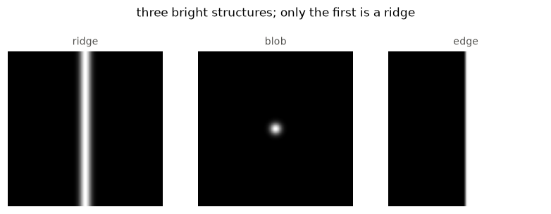

2. Where the eigenvalues come from¶

The filter reads the eigenvalues of the Hessian. The usual reading of $Ax = \lambda x$ does not obviously apply to an image, so this section says what that matrix is and what it acts on.

hessian_matrix convolves the image with the second derivatives of a Gaussian of width σ and returns the upper-triangular entries — in array order $f_{rr}$ , $f_{rc}$ , $f_{cc}$ — as three arrays the size of the image. At one pixel $p$ those three numbers are one symmetric $2 \times 2$ matrix

H_f(p) = \begin{pmatrix} f_{rr}(p) & f_{rc}(p) \\ f_{rc}(p) & f_{cc}(p) \end{pmatrix},

(1)

so the Hessian is one matrix per pixel: a tensor field, a value attached to every point. Each matrix summarises a neighbourhood of size σ, and has its own two eigenvalues. That is the sense in which the eigenvalues are localized.

The table gives the matrix and its eigenvalues at three pixels of one scene.

TILT = 30.0
across = ((rows - MID) * np.sin(np.deg2rad(TILT))
          + (cols - 45) * np.cos(np.deg2rad(TILT)))
scene = (np.exp(-(across**2) / (2 * WIDTH**2))
         + np.exp(-((rows - 55) ** 2 + (cols - 115) ** 2) / (2 * WIDTH**2)))

PROBES = {"ridge crest": (MID, 45), "ridge flank": (54, 70),
          "blob centre": (55, 115)}
elements = hessian_matrix(scene, SIGMA, mode="nearest",
                          use_gaussian_derivatives=True)


def hessian_at(pixel):
    """The 2x2 matrix at one pixel, with its eigenvalues and eigenvectors."""
    f_rr, f_rc, f_cc = (element[pixel] for element in elements)
    matrix = np.array([[f_rr, f_rc], [f_rc, f_cc]])
    values, directions = np.linalg.eigh(matrix)
    order = abs(values).argsort()[::-1]        # largest magnitude first
    return matrix, values[order], directions[:, order]


rows_probe = []
for name, pixel in PROBES.items():
    matrix, values, _ = hessian_at(pixel)
    rows_probe.append({
        "structure": name, "pixel": str(pixel),
        "f_rr": round(matrix[0, 0], 5), "f_rc": round(matrix[0, 1], 5),
        "f_cc": round(matrix[1, 1], 5),
        "λ, larger |·|": round(values[0], 5),
        "λ, smaller |·|": round(values[1], 5),
    })
show_table(pd.DataFrame(rows_probe), index="structure")

The crest has one non-zero curvature and one that vanishes. The flank has the same shape with the opposite sign, because the intensity there curves upward across the ridge. The blob centre curves equally in every direction, so its two eigenvalues are the same number.

The next figure draws each eigenvector at the pixel it belongs to, scaled by its eigenvalue.

LABEL_AT = {"ridge crest": (-26, -20, "right"),
            "ridge flank": (22, 8, "left"),
            "blob centre": (-30, 0, "center")}

fig, ax = plt.subplots(figsize=(5.2, 5.2))
bare(ax)
ax.imshow(scene, cmap="gray")

longest = max(abs(hessian_at(pixel)[1]).max() for pixel in PROBES.values())
for name, pixel in PROBES.items():
    _, values, directions = hessian_at(pixel)
    for value, direction in zip(values, directions.T):
        offset = direction * 20 * abs(value) / longest   # array order: (row, col)
        ax.annotate("", (pixel[1] + offset[1], pixel[0] + offset[0]),
                    (pixel[1] - offset[1], pixel[0] - offset[0]),
                    arrowprops=dict(arrowstyle="<->", lw=1.6, shrinkA=0, shrinkB=0,
                                    color=C_TWO if value < 0 else C_ONE))
    ax.plot(*pixel[::-1], "o", color="white", ms=4, mec=INK, mew=0.8)
    d_row, d_col, align = LABEL_AT[name]
    ax.annotate(name, (pixel[1] + d_col, pixel[0] + d_row), fontsize=7.5,
                color="white", ha=align, va="center")
ax.set_title("eigenvectors at three pixels, scaled by |λ|;\n"
             "orange negative curvature, blue positive", color=MUTED)
fig.tight_layout()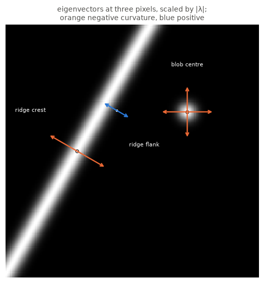

At the crest the long orange arrow points across the ridge and the short one along it — the vanishing eigenvalue has no arrow to speak of. At the blob the two arrows are equal and the axes are arbitrary, which is what a repeated eigenvalue means: every direction is an eigenvector.

The vector such a matrix acts on is a direction in the image plane, of length ndim, not the image. For a unit direction $w$ ,

\kappa(w) = w^{\mathsf T} H_f(p)\, w

(2)

is the curvature of the smoothed intensity surface along $w$ . Turn $w$ through all directions and $\kappa$ traces out a curve with a largest and a smallest value. Those two directions are exactly the eigenvectors of $H_f(p)$ , and the curvatures they attain are the eigenvalues. This is the ordinary eigenvalue problem, with $x$ a direction vector — nothing acts on the image as a vector.

A ridge tilted off the grid axes has all three entries non-zero. Take the crest and compute its eigenvalues three ways:

CREST = PROBES["ridge crest"]
H, values, vectors = hessian_at(CREST)

half_trace = (H[0, 0] + H[1, 1]) / 2
half_root = np.sqrt(H[0, 1] ** 2 + ((H[0, 0] - H[1, 1]) / 2) ** 2)

print("H at the ridge crest:\n", H)
print(f"\nnp.linalg.eigh : {values}")
print(f"skimage        : {hessian_matrix_eigvals(elements)[:, CREST[0], CREST[1]]}")
print(f"closed form    : [{half_trace - half_root:+.6f} {half_trace + half_root:+.6f}]")
print(f"eigenvector angles from the column axis: "
      f"{np.rad2deg(np.arctan2(vectors[0], vectors[1])).round(3)}  (ridge at {TILT}°)")

H at the ridge crest:
 [[-0.008      -0.01385641]
 [-0.01385641 -0.024     ]]

np.linalg.eigh : [-3.20000000e-02 -8.67361738e-19]
skimage        : [ 0.    -0.032]
closed form    : [-0.032000 +0.000000]
eigenvector angles from the column axis: [ 30. -60.]  (ridge at 30.0°)

The eigenvector of the non-zero eigenvalue points at 30°, across the ridge; the other, at −60°, runs along it and reports zero curvature. The three routes agree on the pair. Only the order differs. Those are the notebook’s $u$ and $v$ , and $\lambda_i = v_i^{\mathsf T} H_f v_i$ — used in §4 — is just $\kappa$ read in one of those two directions.

angles = np.linspace(-90, 90, 361)
direction = np.stack([np.sin(np.deg2rad(angles)), np.cos(np.deg2rad(angles))])
curvature = np.einsum("in,ij,jn->n", direction, H, direction)

fig, ax = plt.subplots(figsize=(6.4, 3.0))
ax.plot(angles, curvature, color=C_ONE, lw=1.8)
for value, colour, label in ((values[0], C_TWO, "across the ridge"),
                             (values[1], C_THREE, "along the ridge")):
    ax.axhline(value, color=colour, lw=1.0, ls="--")
    ax.annotate(f"λ = {0.0 if abs(value) < 1e-12 else value:+.3f}, {label}",
                (-88, value), fontsize=7.5,
                color=MUTED, va="bottom")
recede(ax, r"directional curvature $w^\top H_f w$ at one pixel")
ax.set_xlabel("direction of $w$, degrees from the column axis", fontsize=8,
              color=MUTED)
ax.set_xticks([-90, -60, -30, 0, 30, 60, 90])
fig.tight_layout()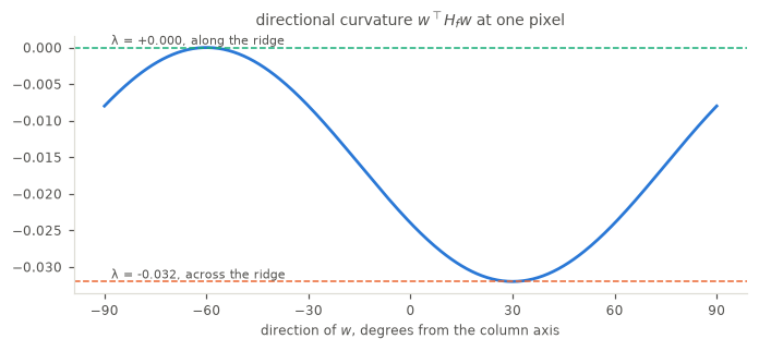

The two eigenvalues are the largest and smallest values of that curve, nothing more.

scikit-image computes them for every pixel at once. In 2-D it uses the closed form above, vectorised over the whole array:

eigs[:] = (M00 + M11) / 2
hsqrtdet = np.sqrt(M01**2 + ((M00 - M11) / 2) ** 2)
eigs[0] += hsqrtdet
eigs[1] -= hsqrtdet

that is $\lambda_\pm = \tfrac12\operatorname{tr} H_f \pm \sqrt{\bigl(\tfrac{f_{rr} - f_{cc}}{2}\bigr)^2 + f_{rc}^2}$ . Above 2-D it assembles the full symmetric matrix per pixel and calls np.linalg.eigvalsh batched over the pixel axes. Either way the result has shape (ndim, *image.shape), the eigenvalue index leading.

print(f"one image of shape {scene.shape} gives eigenvalues of shape "
      f"{hessian_matrix_eigvals(elements).shape}")

one image of shape (161, 161) gives eigenvalues of shape (2, 161, 161)

The eigenvalues come back sorted by signed value, largest first, so the index does not track a fixed geometric role from pixel to pixel. Whatever wants “the principal curvature” must select by magnitude itself, which is what meijering does with abs(vals).argmax(0) in §8.

3. The modified Hessian¶

The paper does not reshape the image or the filter directly. It reshapes the matrix whose eigenvalues are taken. In place of the Hessian $H_f$ it uses

H'_f = \begin{pmatrix} f_{xx} + \alpha f_{yy} & (1-\alpha) f_{xy} \\ (1-\alpha) f_{xy} & f_{yy} + \alpha f_{xx} \end{pmatrix},

(3)

whose eigenvectors are those of $H_f$ and whose eigenvalues are

\lambda'_i = \lambda_i + \alpha \sum_{j \neq i} \lambda_j .

(4)

At $\alpha = 0$ this is the Hessian itself. The paper calls α “a parameter whose optimal value will be given in the sequel”.

scikit-image builds that as a circulant matrix and applies it to the stacked eigenvalues:

mtx = linalg.circulant([1, *[alpha] * (image.ndim - 1)])
vals = np.tensordot(mtx, eigvals, 1)

Check that against the formula, in 2-D and above.

def modified(eigvals, alpha):
    """The paper's lambda'_i, via the circulant scikit-image uses."""
    ndim = len(eigvals)
    return np.tensordot(linalg.circulant([1, *[alpha] * (ndim - 1)]), eigvals, 1)


rng = np.random.default_rng(0)
checks = []
for ndim in (2, 3, 4):
    lam = rng.normal(size=ndim)
    direct = np.array([lam[i] + 0.37 * (lam.sum() - lam[i]) for i in range(ndim)])
    checks.append({"ndim": ndim,
                   "circulant == lambda_i + alpha * sum_{j!=i} lambda_j":
                       bool(np.allclose(modified(lam, 0.37), direct))})
show_table(pd.DataFrame(checks), index="ndim")

4. The filter hiding behind the eigenvalue¶

The appendix of the paper gives the step. $\lambda_i = v_i^{\mathsf T} H_f v_i$ , and that equals $f * (v_i \cdot \nabla)^2 G$ . Read as a function of position, the modified eigenvalue is therefore the output of one convolution, with a reshaped kernel:

\lambda'_i = f * h'_i, \qquad h' = \bigl\{ (r \cdot \nabla)^2 + \alpha (r_\perp \cdot \nabla)^2 \bigr\} G .

(5)

Here $\lambda'_i$ is the whole eigenvalue image, not the number at one pixel, and $r$ is the direction that fixes the kernel. Where the ridge direction changes across the image, the kernel must turn with it.

So α does not merely rescale a number. It picks a filter. Writing $u$ for the direction $r$ and $v$ for $r_\perp$ , and using $G = g(u)g(v)$ ,

h'(u, v) = G_{uu} + \alpha G_{vv} = G \cdot \frac{(u^2 - \sigma^2) + \alpha (v^2 - \sigma^2)}{\sigma^4}.

(6)

def h_prime(alpha, sigma, half, samples=None):
    """Meijering's steerable filter. Axis 0 is across the ridge, axis 1 along."""
    axis = (np.arange(-half, half + 1.0) if samples is None
            else np.linspace(-half, half, samples))
    u, v = np.meshgrid(axis, axis, indexing="ij")
    gauss = np.exp(-(u**2 + v**2) / (2 * sigma**2)) / (2 * np.pi * sigma**2)
    across = gauss * (u**2 - sigma**2) / sigma**4
    along = gauss * (v**2 - sigma**2) / sigma**4
    return axis, across + alpha * along

If the identity holds, convolving an image with h_prime must reproduce the selected modified eigenvalue. A vertical ridge makes that testable, because there the eigenvector directions are known in advance.

def selected_lambda(image, alpha, sigma=SIGMA):
    """What `meijering` computes per scale, before the clip and normalisation."""
    eigvals = hessian_matrix_eigvals(
        hessian_matrix(image, sigma, mode="nearest", use_gaussian_derivatives=True))
    vals = modified(eigvals, alpha)
    return np.take_along_axis(vals, abs(vals).argmax(0)[None], 0).squeeze(0)


interior = slice(20, -20)


def route_gap(alpha, half_widths=8):
    """Eigenvalue route against convolution route, on the ridge's centre row."""
    _, kernel = h_prime(alpha, SIGMA, int(half_widths * SIGMA))
    # The ridge runs down the columns, so "across" is axis 1: transpose.
    by_convolution = ndi.convolve(STRUCTURES["ridge"], kernel.T, mode="nearest")
    by_eigenvalue = selected_lambda(STRUCTURES["ridge"], alpha)
    gap = np.abs(by_eigenvalue[MID][interior] - by_convolution[MID][interior]).max()
    return gap, np.abs(by_convolution[MID]).max()


show_table(
    pd.DataFrame(
    [{"alpha": round(a, 4),
      "max |eigenvalue route − convolution route|": f"{route_gap(a)[0]:.1e}",
      "response scale": f"{route_gap(a)[1]:.1e}"}
     for a in (-1 / 3, 0.0, 1 / 3)]),
    index="alpha",
)

The two routes agree to floating point. The remaining difference is kernel truncation: widen the kernel and it goes away.

show_table(
    pd.DataFrame(
    [{"kernel half-width": f"{m}σ",
      "max gap": f"{route_gap(-1 / 3, m)[0]:.1e}",
      "relative": f"{route_gap(-1 / 3, m)[0] / route_gap(-1 / 3, m)[1]:.1e}"}
     for m in (4, 6, 8, 10)]),
    index="kernel half-width",
)

So α is a knob on the shape of a filter, and the rest of this notebook is about what that shape looks like.

5. The shape α selects¶

The filter can therefore be drawn. This is the paper’s Figure 5, whose caption notes the filter “is more elongated than the filter normally found in the literature on detection of line-like structures” — that literature being $G_{uu}$ alone, which is α = 0.

fig, axes = plt.subplots(1, 4, figsize=(11.0, 3.0))
for ax, (alpha, label) in zip(axes, ((1 / 3, "+1/3  (shipped)"),
                                     (0.0, "0  (plain $G_{uu}$)"),
                                     (-1 / 3, "−1/3  (paper)"),
                                     (-1.0, "−1"))):
    _, kernel = h_prime(alpha, SIGMA, 14, samples=241)
    limit = np.abs(kernel).max()
    bare(ax, f"α = {label}")
    ax.imshow(kernel, cmap=DIV, vmin=-limit, vmax=limit)
    ax.contour(kernel, levels=[0], colors=[INK], linewidths=0.7)
fig.suptitle("$h'$, with its zero contour;  orange negative, blue positive."
             "  The ridge runs left–right", y=1.06)
fig.tight_layout()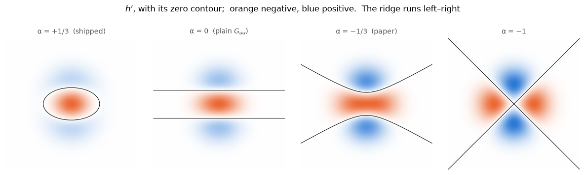

Read left to right, α runs the filter from compact to split. At $+1/3$ the negative core is a closed ellipse — a blob detector. At 0 it is a bar. At $-1/3$ it is longer still, the zero contour bending away from the axis. At -1 the core has split in two and the centre of the filter carries no weight at all, because $h'(0,0) \propto -(1+\alpha)$ vanishes there — tabulated in §7.1.

6. Where −1/3 comes from¶

The paper’s 2-D criterion is that $h'$ be “maximally flat in its longitudinal direction”, written

\lim_{x \to 0} (r_\perp \cdot \nabla)^2 h'(x) = 0 ,

(7)

that is: the filter’s profile along the ridge has no curvature at the centre. Working out the left-hand side with $G = g(u)g(v)$ , $A = g(0)$ , $g''(0) = -A/\sigma^2$ and $g''''(0) = 3A/\sigma^4$ ,

\partial_{vv} h'(0,0) = G_{uuvv}(0) + \alpha G_{vvvv}(0) \propto \frac{1 + 3\alpha}{\sigma^4},

(8)

which is the paper’s $(1 + 3\alpha)\|r\|^4/\sigma^4$ and vanishes at $\alpha = -1/3$ .

For the normalized Gaussian used in the check below, the proportionality constant is $A^2$ .

def longitudinal_curvature(alpha, sigma, half=24):
    """d^2/dv^2 of h' at the origin, evaluated analytically on the grid."""
    axis = np.arange(-half, half + 1.0)
    u, v = np.meshgrid(axis, axis, indexing="ij")
    gauss = np.exp(-(u**2 + v**2) / (2 * sigma**2)) / (2 * np.pi * sigma**2)
    g_uuvv = gauss * (u**2 - sigma**2) * (v**2 - sigma**2) / sigma**8
    g_vvvv = gauss * (v**4 - 6 * sigma**2 * v**2 + 3 * sigma**4) / sigma**8
    return (g_uuvv + alpha * g_vvvv)[half, half]


amplitude = 1 / np.sqrt(2 * np.pi * SIGMA**2)
show_table(
    pd.DataFrame(
    [{"alpha": round(a, 4),
      "grid": f"{longitudinal_curvature(a, SIGMA):+.4e}",
      "closed form  A²(1+3α)/σ⁴":
          f"{amplitude**2 * (1 + 3 * a) / SIGMA**4:+.4e}"}
     for a in (1 / 3, 0.0, -1 / 3, -1.0)]),
    index="alpha",
)

The criterion is the flatness of one curve at one point.

fig, axes = plt.subplots(1, 2, figsize=(10.4, 3.0))

for alpha, colour, label in ((1 / 3, C_TWO, "+1/3"), (0.0, MUTED, "0"),
                             (-1 / 3, C_ONE, "−1/3"), (-1.0, C_THREE, "−1")):
    axis, kernel = h_prime(alpha, SIGMA, 9, samples=201)
    profile = kernel[kernel.shape[0] // 2]
    axes[0].plot(axis, profile / np.abs(profile).max(), color=colour, lw=1.8,
                 label=f"α = {label}")
axes[0].axvline(0, color=GRID, lw=1)
recede(axes[0], "profile along the ridge, $h'(0, v)$, each scaled to its own peak")
axes[0].set_xlabel("distance along the ridge", fontsize=8, color=MUTED)
axes[0].legend(frameon=False, fontsize=8, loc="lower right")

sweep = np.linspace(-1.0, 0.6, 200)
for ndim, colour in ((2, C_ONE), (3, C_TWO), (4, C_THREE)):
    axes[1].plot(sweep, 1 + (ndim + 1) * sweep, color=colour, lw=1.8,
                 label=f"{ndim}-D:  1 + {ndim + 1}α")
    axes[1].plot([-1 / (ndim + 1)], [0], "o", color=colour, ms=6)
axes[1].axhline(0, color=GRID, lw=1)
recede(axes[1], "longitudinal curvature ÷ $A^n/σ^4$;  zero is the criterion")
axes[1].set_xlabel("α", fontsize=8, color=MUTED)
axes[1].legend(frameon=False, fontsize=8)
fig.tight_layout()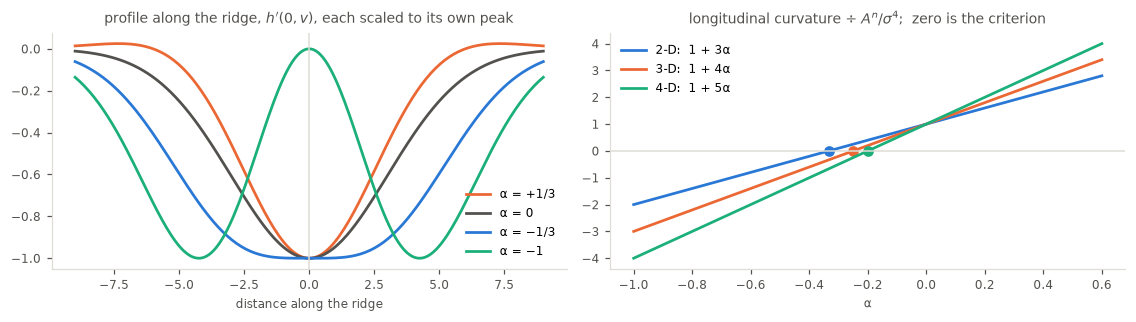

In the left panel the $-1/3$ curve is the one that leaves its minimum most slowly — flat at the centre, which is the criterion. Above it the profile is more sharply peaked; at -1 the centre has become a local maximum and the filter has split.

The right panel is a notebook extension to $n$ dimensions. The paper derives only the 2-D case, and the constant 3 in $(1+3\alpha)$ is not the dimension: it is $g''''(0)/g(0) = 3/\sigma^4$ , the fourth moment of the 1-D Gaussian. Carrying the limit through in $n$ dimensions adds one term per extra perpendicular direction and gives $1 + (n+1)\alpha$ , so the general answer is $\alpha = -1/(n+1)$ — which is what the scikit-image docstring says.

def flatness_alpha(ndim, sigma=1.7):
    """Solve d^2/dv^2 [G_uu + alpha * sum_perp G_kk] = 0 at the origin."""
    g0 = 1 / np.sqrt(2 * np.pi * sigma**2)
    g2 = -g0 / sigma**2
    g4 = 3 * g0 / sigma**4
    constant = g2 * g2 * g0 ** (ndim - 2)                 # G_uuvv(0)
    coefficient = g4 * g0 ** (ndim - 1) + (ndim - 2) * constant
    return -constant / coefficient


show_table(
    pd.DataFrame([{"ndim": n,
               "flatness solve": f"{flatness_alpha(n):+.6f}",
               "-1/(ndim+1)": f"{-1 / (n + 1):+.6f}"} for n in (2, 3, 4, 5)]),
    index="ndim",
)

7. What α does to a ridge, a blob and an edge¶

The shape argument predicts the behaviour. A ridge has one vanishing principal curvature, so $\lambda = (0, \lambda)$ and $\lambda' = (\alpha\lambda, \lambda)$ ; the larger magnitude is $|\lambda|$ for any $|\alpha| < 1$ , independent of α. A step edge has one vanishing curvature too, so the same applies. An isotropic blob centre has $\lambda = (\lambda, \lambda)$ , so $\lambda' = \lambda(1 + \alpha)$ and the response scales as $|1 + \alpha|$ .

WHERE = {"ridge": lambda field: field[MID, MID],
         "blob": lambda field: field[MID, MID],
         "edge": lambda field: field.max()}
alphas = np.linspace(-1.0, 0.6, 33)

responses = {}
for name, image in STRUCTURES.items():
    responses[name] = np.array(
        [WHERE[name](np.maximum(selected_lambda(-image, a), 0)) for a in alphas])

at_zero = responses["blob"][np.argmin(np.abs(alphas))]
predicted = at_zero * np.abs(1 + alphas)

fig, ax = plt.subplots(figsize=(6.4, 3.0))
for name, colour in (("ridge", C_ONE), ("edge", C_THREE), ("blob", C_TWO)):
    ax.plot(alphas, responses[name], color=colour, lw=2.6, alpha=0.55, label=name)
ax.plot(alphas, predicted, color=INK, lw=1.0, ls="--",
        label=r"blob, predicted $\propto |1+\alpha|$")
top = max(responses["blob"].max(), responses["ridge"].max()) * 1.18
for alpha, label in ((1 / 3, "shipped +1/3"), (-1 / 3, "paper −1/3")):
    ax.axvline(alpha, color=GRID, lw=1.1, zorder=0)
    ax.annotate(label, (alpha, top), fontsize=7.5, color=MUTED, ha="center")
ax.set_ylim(-0.002, top * 1.05)
recede(ax, "response against α")
ax.set_xlabel("α", fontsize=8, color=MUTED)
ax.legend(frameon=False, fontsize=8, loc="upper left")
fig.tight_layout()

print(f"ridge response, spread over all α: {np.ptp(responses['ridge']):.2e}")
print(f"edge  response, spread over all α: {np.ptp(responses['edge']):.2e}")
print(f"blob  vs |1+α| law, worst gap:     "
      f"{np.abs(responses['blob'] - predicted).max():.2e}")

blob_at = {a: WHERE["blob"](np.maximum(selected_lambda(-STRUCTURES["blob"], a), 0))
           for a in (1 / 3, -1 / 3)}
print(f"blob at +1/3 over blob at -1/3:    "
      f"{blob_at[1 / 3] / blob_at[-1 / 3]:.4f}   (|(1+1/3)/(1-1/3)| = 2)")

ridge response, spread over all α: 0.00e+00
edge  response, spread over all α: 0.00e+00
blob  vs |1+α| law, worst gap:     6.94e-18
blob at +1/3 over blob at -1/3:    2.0000   (|(1+1/3)/(1-1/3)| = 2)

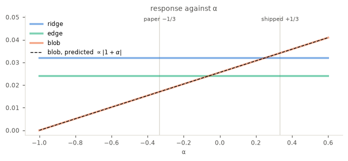
Both flat lines are flat to the last bit, not approximately. For these exact rank-one ridge and edge models, α is a blob dial and nothing else: it acts only where both principal curvatures are non-zero, and leaves those ridges and edges exactly where it found them. Curved, finite, or noisy structures need not have a zero second eigenvalue. The paper’s sign attenuates blobs, the shipped sign amplifies them, by the factor $|(1 + \tfrac13)/(1 - \tfrac13)| = 2$ .

7.1 Why not α = −1?¶

The blob response is exactly zero at $\alpha = -1$ , where $\lambda' = \lambda(1-1)$ , and the ridge response is untouched. On this evidence alone -1 looks strictly better than $-1/3$ .

Section 4 says why it is not: at -1 the filter’s central lobe has split and $h'(0,0) = 0$ . The detector would be reading the image with a kernel that puts no weight at the point it is scoring. The paper’s criterion is a statement about the filter’s shape, not about maximising blob suppression, and the two do not have the same answer.

show_table(
    pd.DataFrame(
    [{"alpha": round(a, 4),
      "h'(0,0)": f"{h_prime(a, SIGMA, 14)[1][14, 14]:+.3e}",
      "longitudinal curvature": f"{longitudinal_curvature(a, SIGMA):+.3e}",
      "blob response": f"{WHERE['blob'](np.maximum(selected_lambda(-STRUCTURES['blob'], a), 0)):.5f}"}
     for a in (1 / 3, 0.0, -1 / 3, -0.6, -1.0)]),
    index="alpha",
)

Only $\alpha = -1/3$ makes the middle column vanish while the first stays well away from zero.

7.2 Off the grid axes¶

The structures in §7 run along the array axes, and the Hessian is computed with axis-aligned separable filters. The argument for α-invariance is about eigenvalues, which are independent of the image orientation. The discrete operator is not. Re-run the claim at angles the grid does not favour.

Build each structure as an exact function of one linear coordinate $d = (r - r_0)\sin\theta + (c - c_0)\cos\theta$ : a Gaussian ridge in $d$ , and an error-function edge in $d$ , which is a smoothed step without a threshold anywhere in its construction.

from scipy import special

MARGIN = 40
ANGLES = (0, 10, 22.5, 30, 45, 63)


def oriented(kind, degrees):
    """A ridge or edge whose normal is `degrees` from the column axis."""
    theta = np.deg2rad(degrees)
    d = (rows - MID) * np.sin(theta) + (cols - MID) * np.cos(theta)
    if kind == "ridge":
        return np.exp(-(d**2) / (2 * WIDTH**2))
    if kind == "edge":
        return 0.5 * (1 + special.erf(d / (WIDTH * np.sqrt(2))))
    # A control: the same edge built by thresholding, then blurring.
    return ndi.gaussian_filter((d >= 0).astype(float), WIDTH)


fig, axes = plt.subplots(2, len(ANGLES), figsize=(11.5, 4.0))
for column, degrees in enumerate(ANGLES):
    for row, kind in enumerate(("ridge", "edge")):
        bare(axes[row, column], f"{kind}, {degrees}°")
        axes[row, column].imshow(oriented(kind, degrees), cmap="gray")
fig.suptitle("rotated test structures: Gaussian ridge (top), erf edge (bottom)",
             y=1.02)
fig.tight_layout()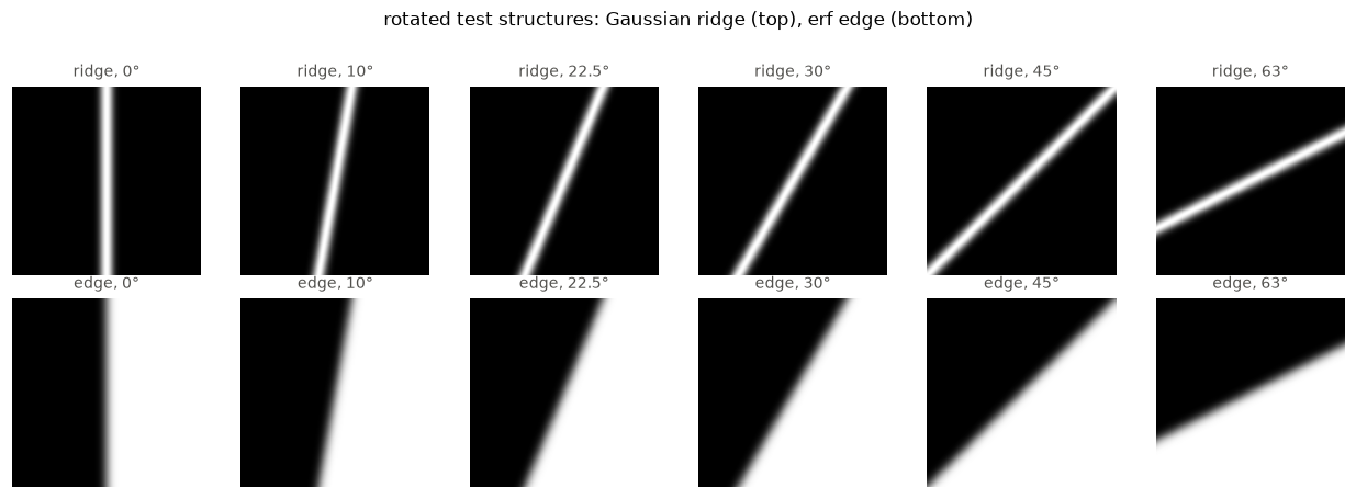

Probe each one at the strongest response, kept away from the frame so the boundary rule cannot contribute, and hold that pixel fixed while α varies.

def interior_probe(field, margin=MARGIN):
    """Brightest pixel, excluding a margin the filter's support cannot cross."""
    window = field[margin:-margin, margin:-margin]
    offset = np.unravel_index(window.argmax(), window.shape)
    return offset[0] + margin, offset[1] + margin


def curvature_ratio(image, probe, sigma=SIGMA):
    """|smaller eigenvalue| / |larger| at one pixel."""
    eigvals = hessian_matrix_eigvals(
        hessian_matrix(-image, sigma, mode="nearest", use_gaussian_derivatives=True))
    eigvals = np.take_along_axis(eigvals, abs(eigvals).argsort(0), 0)
    return abs(eigvals[0][probe]) / abs(eigvals[1][probe])


sweep = np.linspace(-0.8, 0.6, 15)
rows_angle = []
for degrees in ANGLES:
    for kind in ("ridge", "edge", "edge, thresholded"):
        image = oriented(kind, degrees)
        probe = interior_probe(np.maximum(selected_lambda(-image, 0.0), 0))
        values = np.array([np.maximum(selected_lambda(-image, a), 0)[probe]
                           for a in sweep])
        rows_angle.append({
            "degrees": degrees, "structure": kind,
            "|λ₁| / |λ₂|": f"{curvature_ratio(image, probe):.1e}",
            "response": f"{values.mean():.5f}",
            "spread over α, relative": f"{np.ptp(values) / abs(values).mean():.1e}",
        })
show_table(pd.DataFrame(rows_angle), index=["degrees", "structure"])

For the ridge and the erf edge the smaller eigenvalue is zero at every angle, and the response is the same number for every α — 0.0e+00 spread, not a small one. The response magnitude does not move with angle either. α-invariance is not an artefact of axis alignment.

The third row of each block is a control. The same edge built by thresholding d >= 0 and blurring is not a function of $d$ : the threshold staircases along the boundary, which leaves a real second curvature behind, and the invariance breaks at the percent level. Nothing is wrong with the filter there — the test image is not the structure it was meant to be.

worst = {}
for kind in ("ridge", "edge", "edge, thresholded"):
    rel = [float(r["spread over α, relative"]) for r in rows_angle
           if r["structure"] == kind]
    worst[kind] = max(rel)
print("worst relative spread over α, across all angles")
for kind, value in worst.items():
    print(f"  {kind:<20}{value:.1e}")

worst relative spread over α, across all angles
  ridge               0.0e+00
  edge                0.0e+00
  edge, thresholded   1.8e-02

A blob has no orientation to vary, so §7’s $|1+\alpha|$ law needs no rotated counterpart. What the two together say is that α reaches a structure only through the product of its two principal curvatures being non-zero, whatever angle that structure sits at.

8. What scikit-image does¶

The implementation follows the paper closely, with one difference.

if alpha is None:
    alpha = 1 / (image.ndim + 1)                          # <- sign
mtx = linalg.circulant([1, *[alpha] * (image.ndim - 1)])
...
vals = np.tensordot(mtx, eigvals, 1)                      # lambda'_i
vals = np.take_along_axis(vals, abs(vals).argmax(0)[None], 0).squeeze(0)
vals = np.maximum(vals, 0)                                # drop wrong polarity

The circulant is §3’s $\lambda'_i = \lambda_i + \alpha\sum_{j\neq i}\lambda_j$ , verified above. Taking the largest magnitude is the paper’s “λ is the larger in magnitude of the two eigenvalues”, and the clip is its “dark line-like structures, for which λ ≥ 0, are ignored” — after black_ridges has negated the image, if asked.

The magnitude $1/(\mathrm{ndim}+1)$ is §6’s generalisation. The sign is not the paper’s, and not the docstring’s either:

import inspect
from skimage.filters import meijering

source = inspect.getsource(meijering)
doc_line = [line.strip() for line in meijering.__doc__.splitlines()
            if "optimal value" in line]
code_line = [line.strip() for line in source.splitlines()
             if "alpha = " in line and "ndim" in line]
print(f"docstring: {doc_line[0] if doc_line else '(not found)'}")
print(f"code:      {code_line[0] if code_line else '(not found)'}")
print(f"paper (2-D): alpha = -1/3 = {-1 / 3:+.6f}")

docstring: features.  The default, None, selects the optimal value -1/(ndim+1).
code:      alpha = 1 / (image.ndim + 1)
paper (2-D): alpha = -1/3 = -0.333333

on_meijering.md §5.2a measures what that costs, traces it to the ridge-filter rewrite in #6446, and takes up the question of what to do about it. The short version is that $+1/(\mathrm{ndim}+1)$ points the blob dial the wrong way: it turns a suppressor into an amplifier, and answers none of the objection α exists to answer.

9. How to test α¶

meijering_alpha_testing.md takes this section further, and builds a five-test suite around a single picture whose dot and line the filter scores alike when α is switched off. Each test there is stated as a sentence about that picture, and none of them mentions an eigenvalue. What follows is the shorter version, in terms of the quantities this notebook has been working with.

Everything above is also a set of instructions for writing a regression test, and most of the ways such a test goes wrong are ways of accidentally testing something else. The properties worth asserting, and the traps around each:

Assert the invariances, not just the ratio. The ridge and edge responses are exactly α-invariant and the blob scales as $|1+\alpha|$ . A test that only checks the blob is weaker than it looks, because a filter that scaled everything by $|1+\alpha|$ would pass it. Pin both halves.

Beware the per-scale /max. meijering divides each scale by its own maximum before returning, so the brightest structure in the frame is pinned to exactly 1 whatever α does to it. Put one ridge and one blob in an image and the probe you care about is usually that structure — and then an assertion on it cannot fail. Worse, which structure holds the maximum can itself change with α, and then the probe moves for a reason that has nothing to do with the probe.

from skimage.filters import meijering


def probe_and_owner(scene, probe, alpha, sigma=SIGMA):
    """Normalised response at `probe`, and where the per-scale maximum sat."""
    out = meijering(scene, sigmas=[sigma], alpha=alpha, black_ridges=False)
    peak = np.unravel_index(out.argmax(), out.shape)
    return out[probe], peak


small = np.indices((128, 128), dtype=float)
scenes = {
    "ridge + blob, 128 px": (
        np.exp(-((small[1] - 32) ** 2) / (2 * 4.0**2))
        + np.exp(-((small[0] - 64) ** 2 + (small[1] - 64) ** 2) / (2 * 4.0**2)),
        (64, 32), 4.0),
    "ridge + blob, 161 px": (
        np.exp(-((cols - 32) ** 2) / (2 * WIDTH**2))
        + np.exp(-((rows - MID) ** 2 + (cols - MID) ** 2) / (2 * WIDTH**2)),
        (MID, 32), SIGMA),
    "+ a brighter reference ridge": (
        np.exp(-((cols - 32) ** 2) / (2 * WIDTH**2))
        + np.exp(-((rows - MID) ** 2 + (cols - MID) ** 2) / (2 * WIDTH**2))
        + 2 * np.exp(-((cols - 128) ** 2) / (2 * WIDTH**2)),
        (MID, 32), SIGMA),
}

rows_pin = []
for label, (scene, probe, sigma) in scenes.items():
    entry = {"image": label}
    for alpha, name in ((-1 / 3, "α = −1/3"), (1 / 3, "α = +1/3")):
        value, peak = probe_and_owner(scene, probe, alpha, sigma)
        entry[name] = f"{value:.6f}"
        entry[f"max at, {name}"] = str(peak)
    rows_pin.append(entry)
show_table(pd.DataFrame(rows_pin), index="image")

Each of the three images misleads in a different way. In the first the probe ridge reads 1.0 under both signs, because it set the divisor both times: the assertion passes and means nothing. In the second the maximum moves from the ridge to the blob when α flips, so the probe appears to change by 6% — a difference entirely manufactured by the normalisation. Only in the third, where a brighter reference ridge owns the maximum under both signs, is the probe free to move; that it does not is then real evidence.

Either put a dominant reference structure in the frame, or assert on a ratio of two probes, or bypass the normalisation and work with the modified eigenvalues directly as this notebook does.

Use structures that are exact functions of one coordinate. §7.2 is the warning: the invariance belongs to structures whose Hessian is genuinely rank one, and a rotated edge built by thresholding is not one of those. Build ridges as $\exp(-d^2/2w^2)$ and edges as $\operatorname{erf}(d/w\sqrt2)$ , with $d$ linear in the coordinates. Thresholding, drawing with integer endpoints, or rasterising a polygon all reintroduce a second curvature at the percent level, and the test then fails for a reason that has nothing to do with α.

Keep the probe away from the border. mode decides what lies outside the frame, and near the edge that invents curvature the structure does not have. A probe chosen by argmax will find it, given the chance.

diagonal = 0.5 * (1 + special.erf(
    ((rows - MID) * np.sin(np.deg2rad(45)) + (cols - MID) * np.cos(np.deg2rad(45)))
    / (WIDTH * np.sqrt(2))))
field = np.maximum(selected_lambda(-diagonal, 0.0), 0)

naive = np.unravel_index(field.argmax(), field.shape)
guarded = interior_probe(field)
sweep_small = np.linspace(-0.8, 0.6, 9)
gaps = {}
for name, probe in (("argmax anywhere", naive), ("argmax inside a margin", guarded)):
    values = [np.maximum(selected_lambda(-diagonal, a), 0)[probe] for a in sweep_small]
    gaps[name] = {"probe": str(probe),
                  "distance to border": min(probe[0], probe[1],
                                            N - 1 - probe[0], N - 1 - probe[1]),
                  "spread over α": f"{np.ptp(values):.1e}"}
show_table(pd.DataFrame(gaps).T, index=True)

The unguarded probe lands a few pixels from the frame and reports a spread that is entirely the boundary rule. Nothing about α is wrong there; the measurement is.

Choose tolerances from the mechanism, not from habit. The ratio between the two signs is $|(1+\tfrac13)/(1-\tfrac13)| = 2$ exactly, and the measured value departs from it only through the normalisation picking a slightly different maximum pixel. That is a part in 10⁵, so a tolerance of 10^-4 is both safe and four orders sharper than a generic rtol=5e-2 — which would pass even if the ratio were 1.9 or 2.1, values no mechanism here can produce.

Cover every dimension the default is defined for. The default is $-1/(\mathrm{ndim}+1)$ , so 2-D agreement says nothing about 3-D. The cheapest version asserts that alpha=None reproduces the explicit value and does not reproduce its negation, on a small random volume; it needs no model of how 3-D structures behave, which is just as well, because a 3-D line has two non-vanishing curvatures and is not α-invariant the way a 2-D ridge is.

# Scored through `selected_lambda`, not `meijering`: the line is the brightest
# thing in the volume, so the per-scale /max would pin it to 1 and hide this.
zz, yy3, xx3 = np.indices((41, 41, 41), dtype=float)
line_3d = np.exp(-((yy3 - 20) ** 2 + (xx3 - 20) ** 2) / (2 * 3.0**2))
probe_3d = (20, 20, 20)

at_zero_3d = selected_lambda(-line_3d, 0.0, sigma=3.0)[probe_3d]
show_table(
    pd.DataFrame(
    [{"alpha": round(a, 4),
      "3-D line centre": selected_lambda(-line_3d, a, sigma=3.0)[probe_3d],
      "predicted, (1+alpha) x the alpha=0 value": (1 + a) * at_zero_3d}
     for a in (-1 / 4, 0.0, 1 / 4)]).round(8),
    index="alpha",
)

A 2-D ridge has $\lambda = (0, \lambda)$ and the selected $|\lambda'|$ is $|\lambda|$ for any α. A 3-D line has $\lambda = (0, \lambda, \lambda)$ , so $\lambda'_2 = \lambda(1+\alpha)$ and the line does move with α. The 2-D intuition does not transfer, which is another reason to test the default by what it resolves to rather than by what it does.

These are the checks in ../meijering-alpha-fix: test_meijering_default_alpha_suppresses_blobs carries the first four, and test_meijering_default_alpha_is_documented_value is the parametrised dimension check.

10. Summary¶

question	answer	where
eigenvalues of what?	a $2\times2$ matrix per pixel, built from $f_{rr}, f_{rc}, f_{cc}$ ; it acts on directions, not on the image	§2
what is α?	the mixing constant in $\lambda'_i = \lambda_i + \alpha\sum_{j\neq i}\lambda_j$	§3
what does it change?	the shape of the filter $h' = \{(r\cdot\nabla)^2 + \alpha(r_\perp\cdot\nabla)^2\}G$ , since $\lambda'_i = f * h'_i$	§4, §5
why −1/3?	it is the unique α making $h'$ flat along the ridge at the origin, $(1+3\alpha) = 0$	§6
in n dimensions?	notebook extension: $1 + (n+1)\alpha = 0$ , so $-1/(n+1)$	§6
what does it buy?	blob suppression in the tested rank-one models; ridge and edge responses are α-invariant there	§7
why not −1?	blobs vanish, but so does the filter’s centre	§7.1
what does skimage use?	$+1/(\mathrm{ndim}+1)$ , the right magnitude with the wrong sign	§8

Limits. The structures here are synthetic and noise-free, at one σ, scored at the centre of the blob and ridge and at the strongest interior pixel of the edge. The α-invariance of the ridge and edge responses is exact for structures that are functions of a single linear coordinate, which these are by construction, and §7.2 shows that holds at six orientations rather than only along the axes. A curved or finite-length ridge is not such a function, does not have a vanishing second curvature everywhere, and is not tested here — nor is anything with noise, where the smaller eigenvalue is never exactly zero. §7.2’s third row is the reminder that the property belongs to the structure and not to the filter: build the same edge with a threshold and it goes away.

§4’s identity is checked on a vertical ridge, where the eigenvector directions are known in advance; it is not checked where the orientation varies within one image. The 3-D and higher rows of §6’s table are the same limit worked through, not a measurement on 3-D images.

print(f"scikit-image {ski.__version__}")

scikit-image 0.26.1rc0.dev0

References¶

Meijering, E., Jacob, M., Sarria, J. ‐C. F., Steiner, P., Hirling, H., & Unser, M. (2004). Design and validation of a tool for neurite tracing and analysis in fluorescence microscopy images. Cytometry Part A, 58A(2), 167–176. 10.1002/cyto.a.20022