How skimage.draw.line and skimage.draw.line_nd turn a line segment into
pixels, why they disagree, how they compare with Pillow and OpenCV, and what we
could change.
Throughout, coordinates are in array order: the first number indexes the
first array axis, which runs down the picture, and the second indexes the
second axis, which runs right. Nothing here uses x and y.
import itertools

import numpy as np
import matplotlib.pyplot as plt
from matplotlib.patches import Rectangle, Patch
from matplotlib.colors import LinearSegmentedColormap, ListedColormap
from skimage.draw import line, line_ndfatal: not a git repository (or any of the parent directories): .git
fatal: not a git repository (or any of the parent directories): .git
# Comparators.
import cv2
from PIL import Image, ImageDraw
# Slots 1 and 2 of the reference categorical palette, validated as a pair:
# CVD dE 24.7, normal-vision dE 33.6, both well clear of the floors.
C_LINE = "#2a78d6" # skimage.draw.line
C_ND = "#eb6834" # skimage.draw.line_nd
C_BOTH = "#c9c8c1" # pixels that both algorithms choose
C_OFF = "#f2f1ec" # pixels neither chooses
INK = "#0b0b0b"
MUTED = "#52514e"
GRID = "#dedcd5"
plt.rcParams.update(
{
"figure.dpi": 110,
"font.size": 9,
"axes.titlesize": 9,
"axes.titlecolor": MUTED,
"figure.facecolor": "white",
}
)Drawing helpers
One helper draws an empty pixel grid, one fills pixels, one overlays the ideal segment. Everything below is built from these three.
def pixel_axes(ax, shape, title=None):
    """Draw an empty pixel grid, axis 0 downwards and axis 1 rightwards."""
    n_i, n_j = shape
    ax.set_xlim(-0.5, n_j - 0.5)
    ax.set_ylim(n_i - 0.5, -0.5)
    ax.set_xticks(range(n_j))
    ax.set_yticks(range(n_i))
    ax.set_xticks(np.arange(n_j + 1) - 0.5, minor=True)
    ax.set_yticks(np.arange(n_i + 1) - 0.5, minor=True)
    ax.grid(which="minor", color=GRID, linewidth=0.8)
    ax.tick_params(which="both", length=0, labelsize=7, colors=MUTED)
    ax.set_aspect("equal")
    for spine in ax.spines.values():
        spine.set_visible(False)
    if title is not None:
        ax.set_title(title)
    return ax


def fill(ax, pixels, color, alpha=1.0):
    """Fill each ``(axis 0, axis 1)`` pixel in `pixels`."""
    for i, j in sorted(pixels):
        ax.add_patch(
            Rectangle(
                (j - 0.5, i - 0.5),
                1,
                1,
                facecolor=color,
                edgecolor="white",
                linewidth=1.0,
                alpha=alpha,
                zorder=1,
            )
        )
    return ax


def exact(ax, p, q, color=INK):
    """Overlay the ideal segment from `p` to `q`, with its endpoints."""
    ax.plot([p[1], q[1]], [p[0], q[0]], color=color, linewidth=1.4, zorder=3)
    ax.plot([p[1], q[1]], [p[0], q[0]], "o", color=color, markersize=4, zorder=4)
    return ax


def as_set(coords):
    """A tuple of index arrays, as a set of ``(axis 0, axis 1)`` pairs."""
    return set(zip(*(np.asarray(a).tolist() for a in coords)))


def sk_line(p, q):
    return as_set(line(p[0], p[1], q[0], q[1]))


def sk_nd(p, q):
    return as_set(line_nd(p, q, endpoint=True))
1. The problem
Turning a shape described by coordinates into a set of pixels is rasterisation. A segment runs between two pixel centres, and almost every pixel it crosses is crossed only partly, so the rasteriser has to choose which ones to light.
Two classical answers appear in this notebook, and each of our two functions implements one of them. Bresenham’s algorithm walks the pixel grid using integer arithmetic alone, deciding at each step whether to move on the second axis. A digital differential analyser instead samples the line at even intervals and rounds each sample to a pixel. They agree about most segments and disagree about some, which is what this notebook is about.
Here is the segment from (0, 0) to (1, 4), with the pixels whose squares
the ideal segment intersects.
p, q = (0, 0), (1, 4)
shape = (3, 6)
# Pixel squares centred on integer indices: the segment meets these six.
touches = {(0, 0), (0, 1), (0, 2), (1, 2), (1, 3), (1, 4)}

fig, ax = plt.subplots(figsize=(3.6, 2.0))
pixel_axes(ax, shape)
fill(ax, touches, C_OFF)
exact(ax, p, q)
ax.set_title("the segment (0, 0) to (1, 4) and the pixels it touches")
fig.tight_layout()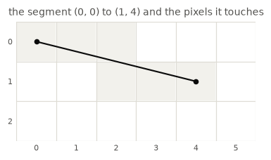
The segment descends one row over four columns, so it passes exactly halfway between two pixel rows at column 2. That single tie is the source of nearly every disagreement in this document.
2. line: integer Bresenham
skimage.draw.line is classic
Bresenham,
implemented in Cython (draw/_draw.pyx::_line). It uses integer arithmetic
only: no floats, no division, and no rounding function anywhere. That was the
point of the algorithm when Bresenham published it in 1965, on hardware where
a division cost far more than an addition, and it is still the reason the
result is exactly reproducible on every machine.
The terms
Four quantities set the problem up.
delta— how far there is to travel on each axis,abs(stop - start).step— which way to travel on each axis,+1or-1.major axis — the axis with the larger
delta. The line advances one pixel along it on every iteration without exception, which is why the output holds exactlydelta[major] + 1pixels.minor axis — the other one. It advances on some iterations and not others. Choosing which is the whole of the algorithm.
Write D for delta[major] and d for delta[minor], so that 0 <= d <= D.
Direction does not enter what follows. The arithmetic below uses delta
alone, which holds absolute distances, and step carries the sign separately.
So the derivation can be read as though the line ran down and to the right,
and a cell after the code confirms that the decisions are identical in every
octant, under transposition and under translation.
The Cython source calls the axes r and c, and physically swaps them when
the line is steep so that the driving axis is always c. Indexing the axes
rather than swapping them says the same thing with less bookkeeping.
The exact line, and the pixel that stands in for it
Two quantities matter, one real and one integer, and the algorithm is entirely about the gap between them.
After k steps along the major axis, the exact line sits at minor
coordinate
y(k) = k * d / Dpixels from the start. That is a real number, and for most k it is not a
whole number of pixels. Nothing can be drawn there.
What is drawn instead is an integer, m(k), measured the same way: whole
pixels from the start along the minor axis. Because the line starts on a pixel,
m(k) is also the number of minor steps taken so far. So each step carries a
discrepancy
y(k) - m(k)between where the line really is and where the pixel had to go. Bresenham’s guarantee is that this stays within
-1/2 <= y(k) - m(k) < 1/2which is to say the drawn pixel is always the nearest one, with an exact tie
resolved by stepping early — taking the higher minor coordinate, so the gap
lands on -1/2 rather than +1/2. The half-open end of that interval is
the tie-breaking rule of section 4, written as mathematics.
Turning the decision into an integer
At step k the algorithm has drawn m(k) and the major axis is about to
advance to k + 1. The two candidates for the next minor coordinate are
m(k) and m(k) + 1, so the line should step when it has passed the midpoint
between them:
step the minor axis <=> y(k + 1) >= m(k) + 1/2Rearranged, the quantity whose sign decides the step is
y(k + 1) - (m(k) + 1/2) = (k + 1) * d / D - m(k) - 1/2This is a fraction, with a division by D and a half. Both can be cleared at
once by multiplying by 2 * D, and because 2 * D is positive the sign — the
only part the test uses — does not change. That product is the error the code
carries:
    error(k)  =  2 * D * [ y(k + 1) - (m(k) + 1/2) ]
              =  2 * (k + 1) * d  -  2 * D * m(k)  -  D
Every term there is an integer. That is the whole of why Bresenham needs no floating point: the decision was never really a fractional question, only a fractional way of writing an integer one.
Two consequences give the code its three constants. Setting k = 0 and
m = 0 gives the starting value
error(0) = 2 * d - Dand subtracting consecutive values gives the update. Writing s for 1 if the
minor axis stepped and 0 if it did not,
error(k + 1) - error(k) = 2 * d - 2 * D * sso each iteration adds 2 * d unconditionally, and subtracts 2 * D as well
whenever it steps.
The algorithm
def bresenham(start, stop):
    """Bresenham's line, in the same steps as `skimage.draw.line`."""
    start, stop = np.array(start), np.array(stop)
    delta = np.abs(stop - start)
    step = np.sign(stop - start)

    major = int(np.argmax(delta))    # the axis with further to travel
    minor = 1 - major

    # `error` is the midpoint test of the previous section, cleared of
    # fractions by the factor 2 * delta[major]:
    #
    #     error(k) = 2 * delta[major] * [ y(k + 1) - (m(k) + 1/2) ]
    #
    # The 2 clears the half, delta[major] clears the division, and both are
    # positive so the sign is untouched. At k = 0 the minor axis has not
    # moved, which leaves the expression below.
    error = 2 * delta[minor] - delta[major]

    at = start.copy()
    pixels = []
    for _ in range(delta[major]):
        pixels.append(tuple(at))

        # error(k + 1) - error(k) = 2 * delta[minor] - 2 * delta[major] * s,
        # where s is 1 when the minor axis steps and 0 when it does not. So
        # the subtraction is conditional and the addition is not.
        if error >= 0:
            at[minor] += step[minor]
            error -= 2 * delta[major]
        at[major] += step[major]
        error += 2 * delta[minor]

    pixels.append(tuple(stop))       # the endpoint is written, never computed
    return pixels
The last line matters: the endpoint is assigned rather than arrived at, so both ends are always present whatever the arithmetic did on the way.
It is the same algorithm
Prose about a reimplementation is worth little. Check it against the real function, over every integer endpoint pair in a 15 by 15 box, comparing the pixel sequence and not merely the set.
R = range(-7, 8)
all_pairs = [((a, b), (c, d)) for a, b, c, d in itertools.product(R, repeat=4)]


def sk_sequence(p, q):
    ii, jj = line(p[0], p[1], q[0], q[1])
    return list(zip(ii.tolist(), jj.tolist()))


matches = sum(bresenham(p, q) == sk_sequence(p, q) for p, q in all_pairs)
print(f"identical to skimage.draw.line on {matches}/{len(all_pairs)} pairs"
      f"  ({matches / len(all_pairs):.1%})")
identical to skimage.draw.line on 50625/50625 pairs (100.0%)
The derivation, checked
Three claims were made above without proof. Each is a statement about every iteration of every line, so each can be tested as one.
The first is that the drawn pixel is always the nearest, ties stepping early —
the interval [-1/2, +1/2).
def discrepancies(start, stop):
    """Per step: k, the exact position, the drawn integer, the gap, the error."""
    start, stop = np.array(start), np.array(stop)
    delta = np.abs(stop - start)
    major = int(np.argmax(delta))
    minor = 1 - major
    d_major, d_minor = int(delta[major]), int(delta[minor])
    if d_major == 0:
        return []

    error, drawn, out = 2 * d_minor - d_major, 0, []
    for k in range(d_major + 1):
        y_exact = k * d_minor / d_major
        out.append((k, y_exact, drawn, y_exact - drawn, error))
        if k == d_major:
            break
        if error >= 0:
            drawn += 1
            error -= 2 * d_major
        error += 2 * d_minor
    return out


gaps = [row[3] for p, q in all_pairs for row in discrepancies(p, q)]
print(f"discrepancy over {len(all_pairs)} lines: [{min(gaps)}, {max(gaps)})")
print(f"   never below -1/2 : {min(gaps) >= -0.5}")
print(f"   always below 1/2 : {max(gaps) < 0.5}")

print(f"\nthe tie case, (0, 0) to (1, 4):")
print(f"{'k':>4}{'y(k) exact':>13}{'m(k) drawn':>13}{'gap':>8}{'error':>8}")
for k, y_exact, drawn, gap, err in discrepancies((0, 0), (1, 4)):
    print(f"{k:>4}{y_exact:>13.2f}{drawn:>13}{gap:>8.2f}{err:>8}")
discrepancy over 50625 lines: [-0.5, 0.4615384615384617)
never below -1/2 : True
   always below 1/2 : True

the tie case, (0, 0) to (1, 4):
   k   y(k) exact   m(k) drawn     gap   error
   0         0.00            0    0.00      -2
   1         0.25            0    0.25       0
   2         0.50            1   -0.50      -6
   3         0.75            1   -0.25      -4
   4         1.00            1    0.00      -2
The -0.5 in that last line is the tie, and it is reached rather than avoided:
an exact half steps early.
The second claim is the closed form for error(k) itself.
def error_matches_closed_form(start, stop):
    """Is `error` equal to 2 * D * [y(k + 1) - (m(k) + 1/2)] at every step?"""
    start, stop = np.array(start), np.array(stop)
    delta = np.abs(stop - start)
    major = int(np.argmax(delta))
    minor = 1 - major
    d_major, d_minor = int(delta[major]), int(delta[minor])

    error, drawn = 2 * d_minor - d_major, 0
    for k in range(d_major):
        closed_form = 2 * d_major * ((k + 1) * d_minor / d_major - drawn - 0.5)
        if abs(error - closed_form) > 1e-9:
            return False
        if error >= 0:
            error -= 2 * d_major
            drawn += 1
        error += 2 * d_minor
    return True


agree = sum(error_matches_closed_form(p, q) for p, q in all_pairs)
print(f"error matches the closed form on {agree}/{len(all_pairs)} pairs")
error matches the closed form on 50625/50625 pairs
The third is that direction never enters, so reading the derivation in one octant was safe.
def decisions(start, stop):
    """The error sequence alone, with no positions."""
    start, stop = np.array(start), np.array(stop)
    delta = np.abs(stop - start)
    d_major, d_minor = int(delta.max()), int(delta.min())
    error, out = 2 * d_minor - d_major, []
    for _ in range(d_major):
        out.append(error)
        if error >= 0:
            error -= 2 * d_major
        error += 2 * d_minor
    return out


base = decisions((0, 0), (2, 7))
elsewhere = {
    "up and left, (-2, -7)": ((0, 0), (-2, -7)),
    "down and left, (2, -7)": ((0, 0), (2, -7)),
    "transposed, (7, 2)": ((0, 0), (7, 2)),
    "translated by (5, 5)": ((5, 5), (7, 12)),
}
for name, (start, stop) in elsewhere.items():
    print(f"{name:<24} same error sequence as (2, 7): "
          f"{decisions(start, stop) == base}")
up and left, (-2, -7) same error sequence as (2, 7): True
down and left, (2, -7) same error sequence as (2, 7): True
transposed, (7, 2) same error sequence as (2, 7): True
translated by (5, 5) same error sequence as (2, 7): True
Why one minor step is always enough
The Cython source writes the decision as while d >= 0, not if. The two are
the same here: the minor axis never has further to travel than the major one,
so it can never need two steps in one iteration. Since that is what licenses
the if above, check it rather than assume it.
def never_steps_twice(start, stop):
    """Would a second pass of the `while` body ever be taken?"""
    start, stop = np.array(start), np.array(stop)
    delta = np.abs(stop - start)
    d_major, d_minor = int(delta.max()), int(delta.min())
    error = 2 * d_minor - d_major
    for _ in range(d_major):
        if error >= 0:
            error -= 2 * d_major
            if error >= 0:
                return False
        error += 2 * d_minor
    return True


single = sum(never_steps_twice(p, q) for p, q in all_pairs)
print(f"one minor step per major step suffices on {single}/{len(all_pairs)} pairs")
one minor step per major step suffices on 50625/50625 pairs
And the line it draws:
fig, ax = plt.subplots(figsize=(3.6, 2.0))
pixel_axes(ax, shape)
fill(ax, sk_line(p, q), C_LINE)
exact(ax, p, q, color="white")
ax.set_title("line(0, 0, 1, 4)")
fig.tight_layout()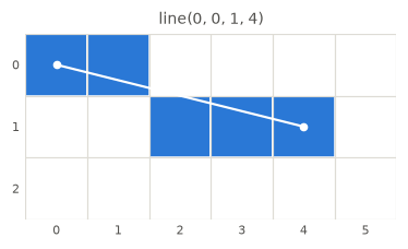
3. line_nd: sample, then round each axis
skimage.draw.line_nd (draw/draw_nd.py) works differently. It computes how
many points it needs, samples the segment at that many equally spaced
parameters with np.linspace, and then rounds each axis independently.
That is a digital differential analyser: step along the line in equal increments and round. The approach costs floating point arithmetic that Bresenham avoids, and buys two things Bresenham cannot offer — any number of dimensions, and endpoints that need not be integers.
It is also the textbook definition of digitising a curve.
Knuth (1990) sets it out for any parametric
path z(t) = (x(t), y(t)) as
round z(t) = (round x(t), round y(t))“as t varies, where round(a) is the integer nearest a” — which is exactly
what line_nd computes, one axis at a time. So line_nd is not an ad hoc
choice; it is the standard digitisation, and the interesting question is what it
does at the one place that definition does not reach.
npoints = ceil(max(abs(stop - start)))
coords  = linspace(start, stop, npoints).T
coords  = round(coords)        # per axis, via _round_safe
The rounding is np.round, which sends a half to the nearest even integer,
so 0.5 becomes 0 while 1.5 becomes 2. Rounding each axis independently
can then open a two-pixel gap between consecutive samples, and _round_safe
guards against that one case by falling back to np.floor.
Knuth reaches the same fork and declines to take it. Immediately after giving
the rule he writes that “we need to be careful, of course, when rounding values
that are halfway between integers, because round(a) is undefined in such
cases”, and then assumes the path never passes through a pixel centre: exact
hits “occur with probability zero”, and “an infinitesimal shift of the path can
be used to avoid pixel centers in general, therefore avoiding the ambiguities
pointed out in Bresenham’s interesting discussion”.
So the tie is not an oversight in the definition. It is the one case the
definition leaves open, flagged as such, with a pointer to the paper that works
through the consequences. _round_safe is skimage meeting that case in
practice, where “probability zero” is not available: integer endpoints put the
midpoint of an odd-length run exactly on a half every time. Section 10 comes
back to what Knuth’s infinitesimal shift means for the choice of rounding rule.
How one coordinate breaks the whole line
np.round([0.5, 1.5]) == [0, 2] is a fact about two numbers. Getting from there
to a hole in a drawn line takes three steps.
A line is connected when consecutive pixels touch. line_nd documents
ndim-connectivity: “two subsequent pixels in the line will be either direct or
diagonal neighbors”. Neighbours differ by at most 1 in every axis, so
connectivity is a condition on all the axes at once. It therefore fails if any
single axis jumps by 2. The other axes cannot make up for it — a pixel two
rows away is not a neighbour whatever the columns do.
Before rounding, the samples are already close enough. npoints comes from
the largest of the deltas, so the axis with furthest to travel advances exactly
1 per sample and every other axis advances less. The chain of real-valued
samples is connected with room to spare. Every gap is made by the rounding.
Rounding moves each sample by at most half a pixel. So two samples exactly 1
apart can land at most 1 + 1/2 + 1/2 = 2 apart. Reaching 2 needs both halves
of that slack, which means the first sample must round down by exactly a
half and the second up by exactly a half. Only exact halves round by exactly
a half, so both samples must be halves, and they must round in opposite
directions.
Half-to-even supplies both conditions at once. Which way it rounds a half depends on which neighbour is even, and that alternates from one half to the next:
print(f"{'sample':>8}{'rounds to':>12}{'direction':>12}{'error':>9}"
      f"{'because':>28}")
for value in (0.5, 1.5, 2.5, 3.5):
    got = np.round(value)
    below, above = int(np.floor(value)), int(np.ceil(value))
    even = below if below % 2 == 0 else above
    print(f"{value:>8}{got:>12.0f}{'down' if got < value else 'up':>12}"
          f"{got - value:>+9.1f}{f'{even} is the even neighbour':>28}")
sample rounds to direction error because
0.5 0 down -0.5 0 is the even neighbour
1.5 2 up +0.5 2 is the even neighbour
2.5 2 down -0.5 2 is the even neighbour
3.5 4 up +0.5 4 is the even neighbour
So consecutive halves round alternately down, up, down, up — which is exactly the down-then-up pattern a two-pixel jump requires. Two consecutive halves on one axis are all it takes.
The geometry says the same thing in one sentence. A sample at row 0.5 sits
exactly on the boundary between rows 0 and 1, touching both; the next sample, at
row 1.5, sits on the boundary between rows 1 and 2. Row 1 is the row they
have in common. Half-to-even sends the first sample to row 0 and the second to
row 2, so row 1 is skipped — the exact line crosses it, and no pixel of it is
ever drawn.
gap_start, gap_stop = (0.5, 0.0), (3.5, 3.0)
gap_samples = np.linspace(gap_start, gap_stop, 4)
gap_rows, gap_cols = gap_samples[:, 0], gap_samples[:, 1]

to_even = [(int(np.round(r)), int(c)) for r, c in gap_samples]
to_up = [(int(np.floor(r + 0.5)), int(c)) for r, c in gap_samples]
SHAPE_ROWS, SHAPE_COLS = 5, 4
SHAPE = (SHAPE_ROWS, SHAPE_COLS)

drawn_rows = {row for row, _ in to_even}
skipped_rows = [r for r in range(SHAPE_ROWS) if r not in drawn_rows]

fig, axes = plt.subplots(1, 3, figsize=(9.6, 2.9))

pixel_axes(axes[0], SHAPE, "every sample lands on a row boundary")
for boundary in (0.5, 1.5, 2.5, 3.5):
    axes[0].axhline(boundary, color=C_LINE, lw=1.4, ls="--", zorder=2)
exact(axes[0], gap_start, gap_stop, color=INK)
axes[0].plot(gap_cols, gap_rows, "o", color=INK, markersize=5, zorder=6)
for row, col in gap_samples:
    axes[0].annotate(f"row {row:g}", (col, row), textcoords="offset points",
                     xytext=(8, 9), fontsize=7, color=C_LINE, zorder=7,
                     bbox=dict(boxstyle="round,pad=0.15", fc="white", ec="none"))

pixel_axes(axes[1], SHAPE, "half to even: rows 0, 2, 2, 4")
fill(axes[1], to_even, C_ND)
for row in skipped_rows:
    axes[1].add_patch(Rectangle((-0.5, row - 0.5), SHAPE_COLS, 1, facecolor="none",
                                edgecolor=C_LINE, lw=1.6, ls=":", zorder=5))
exact(axes[1], gap_start, gap_stop, color=INK)

pixel_axes(axes[2], SHAPE, "half up: rows 1, 2, 3, 4")
fill(axes[2], to_up, C_ND)
exact(axes[2], gap_start, gap_stop, color=INK)

fig.suptitle("dotted band: a row the line crosses and no pixel is drawn in",
             y=1.03)
fig.tight_layout()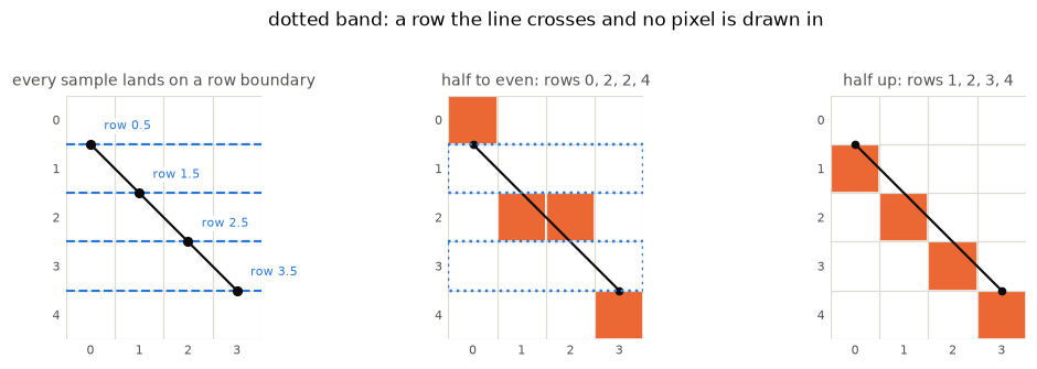
The middle panel is not one line but three pieces — a lone pixel, an adjacent pair, and another lone pixel — separated by the two dotted rows. The right panel is the same segment with the ties resolved one fixed way instead of alternately, and it is a single connected chain.
from skimage.measure import label

for name, pixels in (("half to even", to_even), ("half up", to_up)):
    canvas = np.zeros(SHAPE, int)
    for row, col in pixels:
        canvas[row, col] = 1
    print(f"   {name:<14}{label(canvas, connectivity=2).max()} connected "
          f"component(s) for {len(pixels)} pixels")
half to even 3 connected component(s) for 4 pixels
half up 1 connected component(s) for 4 pixels
The step of exactly 1 is doing real work in that argument, and it confines the whole problem to the axis with furthest to travel. Halve the spacing and the halves stop being consecutive: an integer-valued sample falls between them, rounds to itself, and anchors the chain.
print(f"{'samples on one axis':<44}{'rounded':<22}{'worst step':>11}")
for label, seq in (
    ("spacing 1, starting on a half", np.arange(0.5, 4.5, 1.0)),
    ("spacing 1/2, starting on a half", np.arange(0.5, 3.0, 0.5)),
    ("spacing 1, starting on an integer", np.arange(0.0, 4.0, 1.0)),
    ("spacing 3/4, starting on a half", 0.5 + 0.75 * np.arange(5)),
):
    rounded = np.round(seq).astype(int)
    print(f"   {label:<41}{str(rounded):<22}{np.abs(np.diff(rounded)).max():>11}")
samples on one axis rounded worst step
spacing 1, starting on a half [0 2 2 4] 2
spacing 1/2, starting on a half [0 1 2 2 2] 1
spacing 1, starting on an integer [0 1 2 3] 1
spacing 3/4, starting on a half [0 1 2 3 4] 1
Only the first row can gap, and it needs both a half fraction and a unit step.
That pair of conditions is what _round_safe tests.
Its test is coords[0] % 1 == 0.5 and coords[1] - coords[0] == 1. The first
half is a fractional part of exactly .5, so it holds at any whole number
and not only at 0.5:
def guard_fires(first, spacing=1.0, n=5):
    """The `_round_safe` test, transcribed: a half fraction and unit spacing."""
    coords = first + np.arange(n) * spacing
    return bool(coords[0] % 1 == 0.5 and coords[1] - coords[0] == 1)


print("spacing 1, varying the first coordinate")
for first in (0.0, 0.25, 0.5, 1.5, 3.5, 7.5, -0.5, -2.5):
    print(f"   first = {first:>5}  -> {'floor' if guard_fires(first) else 'round'}")

print("\nfirst coordinate 3.5, varying the spacing")
for spacing in (1.0, 0.999999, 0.5, 2.0):
    print(f"   spacing = {spacing:<9} -> "
          f"{'floor' if guard_fires(3.5, spacing) else 'round'}")
spacing 1, varying the first coordinate
first = 0.0 -> round
first = 0.25 -> round
first = 0.5 -> floor
first = 1.5 -> floor
first = 3.5 -> floor
first = 7.5 -> floor
first = -0.5 -> floor
first = -2.5 -> floor
first coordinate 3.5, varying the spacing
spacing = 1.0 -> floor
spacing = 0.999999 -> round
spacing = 0.5 -> round
spacing = 2.0 -> round
Both conditions have to hold. The spacing is exactly 1 only on the axis with
furthest to travel. Integer endpoints can still put a mid-run sample on a
half — column 2 of (0, 0) to (1, 4) is exactly row 0.5 — but the guard
only inspects coords[0], the first sample, which is then an integer. So the
first half of the test fails, the guard never fires, and line_nd is exactly
np.round of its own samples. That can be checked without touching the
private function at all.
def plain_round(start, stop):
    """What `line_nd` would give if it always used `np.round`."""
    npoints = int(np.ceil(np.max(np.abs(np.subtract(stop, start))))) + 1
    samples = np.linspace(start, stop, npoints, endpoint=True).T
    return [tuple(int(x) for x in c) for c in np.round(samples).astype(int).T]


def nd_pixels(start, stop):
    return [tuple(int(x) for x in c)
            for c in zip(*line_nd(start, stop, endpoint=True))]


distinct = [(a, b) for a, b in all_pairs if a != b]
same = sum(nd_pixels(a, b) == plain_round(a, b) for a, b in distinct)
print(f"integer endpoints: line_nd equals plain np.round on "
      f"{same}/{len(distinct)} pairs  ({same / len(distinct):.1%})")
integer endpoints: line_nd equals plain np.round on 50400/50400 pairs (100.0%)
Where the guard does fire, it earns its place. Starting an axis on a half and
rounding to even makes np.round jump two pixels at a time:
half_start, half_stop = (0.5, 0.0), (4.5, 2.0)
print(f"from {half_start} to {half_stop}")
print(f"   line_nd    {nd_pixels(half_start, half_stop)}")
print(f"   np.round   {plain_round(half_start, half_stop)}")
from (0.5, 0.0) to (4.5, 2.0)
line_nd [(0, 0), (1, 0), (2, 1), (3, 2), (4, 2)]
np.round [(0, 0), (2, 0), (2, 1), (4, 2), (4, 2)]
The second row steps 0, 2, 2, 4, 4 down the first axis, leaving gaps. That is
the two-pixel jump the guard exists to prevent.
The guard only looks one way
The spacing half of the test is coords[1] - coords[0] == 1, and that 1 is
signed. An axis that counts down through the same halves is spaced by -1,
so the test fails and the guard says nothing — even though the samples are
exactly the configuration it was written for.
ends = ((3.5, 0.0), (0.5, 3.0))

for name, (a, b) in (("named down", ends), ("named up", ends[::-1])):
    pixels = nd_pixels(a, b)
    steps = [int(np.max(np.abs(np.subtract(t, s))))
             for s, t in zip(pixels, pixels[1:])]
    print(f"{name}:  {a} -> {b}")
    print(f"   samples on axis 0   {np.linspace(a, b, 4)[:, 0]}")
    print(f"   line_nd             {pixels}")
    print(f"   steps between them  {steps}")
named down: (3.5, 0.0) -> (0.5, 3.0)
samples on axis 0 [3.5 2.5 1.5 0.5]
line_nd [(4, 0), (2, 1), (2, 2), (0, 3)]
steps between them [2, 1, 2]
named up: (0.5, 3.0) -> (3.5, 0.0)
samples on axis 0 [0.5 1.5 2.5 3.5]
line_nd [(0, 3), (1, 2), (2, 1), (3, 0)]
steps between them [1, 1, 1]
One segment, named each way round. Counting up, axis 0 samples
0.5, 1.5, 2.5, 3.5, the guard fires, np.floor gives 0, 1, 2, 3, and the
line is 8-connected. Counting down it samples the very same four halves in the
opposite order, the guard stays silent, np.round sends them to 4, 2, 2, 0,
and the line breaks into three pieces.
fig, axes = plt.subplots(1, 2, figsize=(6.0, 2.6))
for ax, (a, b) in zip(axes, (ends, ends[::-1])):
    pixel_axes(ax, (5, 4), f"{a} to {b}")
    fill(ax, sk_nd(a, b), C_ND)
    exact(ax, a, b, color=INK)
fig.suptitle("line_nd on one segment, named each way round", y=1.02)
fig.tight_layout()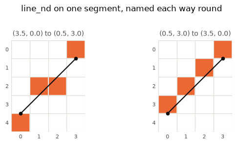
The left panel is not a tie-breaking quirk that costs a pixel here or there: it
is a line with two holes in it. It also costs line_nd the one symmetry
section 6 measured it as holding — over integer endpoints the reversal is
exact, and here it is not.
The case is common rather than rare, because half-integer endpoints are exactly what a caller passing floats tends to produce.
rng = np.random.default_rng(0)
counts = {"every axis counts up": [0, 0], "some axis counts down": [0, 0]}

for _ in range(10000):
    a = rng.integers(0, 20, 2) + 0.5
    b = rng.integers(0, 20, 2) + 0.5
    if np.array_equal(a, b):
        continue
    key = "every axis counts up" if np.all(b >= a) else "some axis counts down"
    pixels = nd_pixels(a, b)
    counts[key][0] += any(np.max(np.abs(np.subtract(t, s))) > 1
                          for s, t in zip(pixels, pixels[1:]))
    counts[key][1] += 1

print("random half-integer endpoints in a 20x20 box")
for key, (bad, total) in counts.items():
    print(f"   {key:<24}{bad:>6} gapped /{total:>6}")
random half-integer endpoints in a 20x20 box
every axis counts up 0 gapped / 2707
some axis counts down 5100 gapped / 7271
Nothing in the guard is direction-aware except that one comparison. The
fractional-part half of the test, coords[0] % 1 == 0.5, holds whichever way
the axis runs, and the docstring reasons only in the ascending direction — its
worked examples are np.arange(0.5, 8, 1) and [0.5, 1.25, 2., 2.75, 3.5],
both counting up. It reads as an oversight rather than a decision.
The pull request that added line_nd,
#2043, supports that
reading twice over. Its opening post proposes the guard as
np.all(arr % 1 == 0.5)over all the coordinates, where the merged code tests only coords[0]; and
it describes the remedy as replacing “round with floor (ie rounding towards
0)”, which np.floor is not — it rounds towards minus infinity, and the two
differ for exactly the descending values that turn out to break. The ascending
mental model is visible in the original wording, before any code was written.
Testing abs(coords[1] - coords[0]) == 1 would close this particular hole;
section 10 argues for removing the need for the guard instead.
So every rounding in the rest of this notebook is plain np.round, half-to-even
and all. _round_safe never comes into it, and the tie behaviour of section 4
is np.round alone.
endpoint is False by default, so the stop point is left out unless asked
for. Every comparison below passes endpoint=True so the point counts match.
samples = np.linspace(p, q, 5, endpoint=True)

fig, ax = plt.subplots(figsize=(3.6, 2.0))
pixel_axes(ax, shape)
fill(ax, sk_nd(p, q), C_ND)
exact(ax, p, q, color="white")
ax.plot(samples[:, 1], samples[:, 0], "o", color=INK, markersize=5, zorder=5)
for i, j in samples:
    ax.annotate(
        f"{i:g}",
        (j, i),
        textcoords="offset points",
        xytext=(0, 9),
        ha="center",
        fontsize=7,
        color=INK,
    )
ax.set_title("line_nd((0, 0), (1, 4)) with its sample points, labelled by exact row")
fig.tight_layout()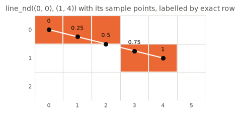
The label on the middle sample is the whole story: the exact row there is
0.5, an exact tie.
print(f"{'column':>7}{'exact row':>11}{'line':>7}{'line_nd':>9}")
lr = dict(zip(*[a.tolist() for a in line(0, 0, 1, 4)][::-1]))
nr = dict(zip(*[a.tolist() for a in line_nd(p, q, endpoint=True)][::-1]))
for j in range(5):
    print(f"{j:>7}{0 + j * 0.25:>11.2f}{lr[j]:>7}{nr[j]:>9}")
column exact row line line_nd
0 0.00 0 0
1 0.25 0 0
2 0.50 1 0
3 0.75 1 1
4 1.00 1 1
4. The tie, side by side
fig, axes = plt.subplots(1, 2, figsize=(7.2, 2.1))
for ax, pix, color, name in (
    (axes[0], sk_line(p, q), C_LINE, "line"),
    (axes[1], sk_nd(p, q), C_ND, "line_nd"),
):
    pixel_axes(ax, shape, name)
    fill(ax, pix, color)
    exact(ax, p, q, color="white")
fig.suptitle("at the tie, line steps early and line_nd steps late", y=1.02)
fig.tight_layout()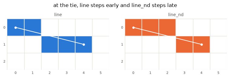
Bresenham’s d >= 0 test resolves the tie by stepping early. np.round
sends 0.5 to 0, so line_nd steps late.
5. How often do they disagree?
Fix the start at the top-left corner and vary the end over a box. Each cell is coloured by whether the two functions produce the same pixels for that endpoint.
n = 13
agree = np.zeros((n, n), dtype=int)
for i in range(n):
    for j in range(n):
        agree[i, j] = sk_line((0, 0), (i, j)) == sk_nd((0, 0), (i, j))

fig, ax = plt.subplots(figsize=(3.4, 3.4))
ax.imshow(agree, cmap=ListedColormap([C_ND, C_OFF]), vmin=0, vmax=1)
ax.set_xticks(range(0, n, 2))
ax.set_yticks(range(0, n, 2))
ax.tick_params(length=0, labelsize=7, colors=MUTED)
for spine in ax.spines.values():
    spine.set_visible(False)
ax.set_xlabel("end, axis 1", fontsize=8, color=MUTED)
ax.set_ylabel("end, axis 0", fontsize=8, color=MUTED)
ax.set_title("start fixed at (0, 0)")
fig.legend(
    handles=[
        Patch(facecolor=C_OFF, label="same pixels"),
        Patch(facecolor=C_ND, label="different pixels"),
    ],
    loc="lower center",
    ncols=2,
    frameon=False,
    fontsize=8,
)
fig.tight_layout(rect=(0, 0.08, 1, 1))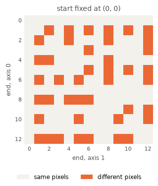
The disagreements are not scattered: they lie along the directions whose slope puts a sample exactly on a half. Over every integer endpoint pair in a 9x9 box, not just those from one corner:
# Every ordered pair of endpoints in a 9x9 box, kept clear of the canvas edge
# so that Pillow and OpenCV have room to draw in section 7.
LO, HI = 4, 13
pts = list(itertools.product(range(LO, HI), repeat=2))
box = [(a, b) for a in pts for b in pts]

diff = sum(sk_line(a, b) != sk_nd(a, b) for a, b in box)
print(f"{len(box)} endpoint pairs, {diff} differ  ({diff / len(box):.1%})")

# The rate depends on the box: longer segments have more chances to hit a tie.
wide = range(-6, 7)
wide_pairs = [((a, b), (c, d)) for a, b, c, d in itertools.product(wide, repeat=4)]
wdiff = sum(sk_line(a, b) != sk_nd(a, b) for a, b in wide_pairs)
print(f"{len(wide_pairs)} pairs in a 13x13 box, {wdiff} differ  ({wdiff / len(wide_pairs):.1%})")
6561 endpoint pairs, 1272 differ (19.4%)
28561 pairs in a 13x13 box, 6000 differ (21.0%)
6. Two symmetries, one each
A rasteriser can have two properties that users assume without thinking.
Translation invariance
Move the segment by a whole number of pixels and the drawn shape should just move with it.
fig, axes = plt.subplots(2, 4, figsize=(9.6, 4.0))
for col, t in enumerate(range(4)):
    a, b = (t, 0), (1 + t, 4)
    for row, (f, color, name) in enumerate(
        ((sk_line, C_LINE, "line"), (sk_nd, C_ND, "line_nd"))
    ):
        ax = axes[row, col]
        pixel_axes(ax, (6, 6), f"{name}, shifted by {t}")
        fill(ax, f(a, b), color)
        exact(ax, a, b, color="white")
fig.suptitle(
    "shift the same segment down one row at a time: line keeps its shape, "
    "line_nd does not",
    y=1.01,
)
fig.tight_layout()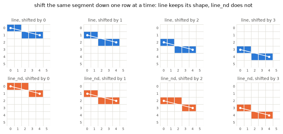
Look along the bottom row. The line_nd shape flips between stepping early and
stepping late as the segment moves, because np.round sends 0.5 to 0 but
1.5 to 2 — half-to-even depends on the parity of the coordinate.
Reversal symmetry
Naming the ends in the other order should draw the same pixels.
This is the older of the two questions. Bresenham (1987) devotes a paper to it: an implementation must “resolve ties in which two candidate grid points have an equal error metric”, and “equal error metric ambiguity can permit algorithmic selection of raster points for a line to differ depending on the direction it is drawn”. That is the defect measured below, named by the author of the algorithm twenty-five years after he published it.
fig, axes = plt.subplots(1, 4, figsize=(9.6, 2.1))
panels = [
    (sk_line, p, q, C_LINE, "line, start to stop"),
    (sk_line, q, p, C_LINE, "line, stop to start"),
    (sk_nd, p, q, C_ND, "line_nd, start to stop"),
    (sk_nd, q, p, C_ND, "line_nd, stop to start"),
]
for ax, (f, a, b, color, name) in zip(axes, panels):
    pixel_axes(ax, shape, name)
    fill(ax, f(a, b), color)
    exact(ax, a, b, color="white")
fig.suptitle("line changes when you swap the ends; line_nd does not", y=1.04)
fig.tight_layout()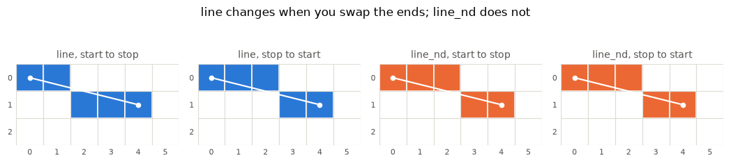
Measured over the whole box:
def symmetry(f, pairs, kind, shift=3):
    ok = 0
    for a, b in pairs:
        if kind == "reversal":
            ok += f(a, b) == f(b, a)
        else:
            moved = {(i + shift, j + shift) for i, j in f(a, b)}
            at = (a[0] + shift, a[1] + shift), (b[0] + shift, b[1] + shift)
            ok += moved == f(*at)
    return ok / len(pairs)


print(f"{'':16}{'reversal':>12}{'translation':>14}")
for name, f in (("line", sk_line), ("line_nd", sk_nd)):
    print(
        f"{name:<16}{symmetry(f, box, 'reversal'):>11.1%}"
        f"{symmetry(f, box, 'translation'):>13.1%}"
    )
reversal translation
line 69.5% 100.0%
line_nd 100.0% 69.5%
Each function holds one property and loses the other.
The line_nd column is a statement about box, which holds integer endpoints.
Its reversal symmetry does not survive half-integer ones: the rounding guard of
section 3 fires on an ascending axis and not on a descending one, so naming the
ends the other way round can change the pixels, and can open a gap.
7. Pillow and OpenCV
Two other widely used rasterisers, for comparison. Both take coordinates in
(column, row) order, so the wrappers below swap.
CANVAS = 24


def pil_line(a, b):
    im = Image.new("L", (CANVAS, CANVAS), 0)
    ImageDraw.Draw(im).line([(a[1], a[0]), (b[1], b[0])], fill=255, width=1)
    return set(map(tuple, np.argwhere(np.array(im))))


def cv_line(a, b, connectivity=8):
    arr = np.zeros((CANVAS, CANVAS), np.uint8)
    cv2.line(arr, (a[1], a[0]), (b[1], b[0]), 255, 1, lineType=connectivity)
    return {(int(i), int(j)) for i, j in np.argwhere(arr)}
off = (4, 4) # keep the segment inside the canvas
pa, qa = (off[0] + p[0], off[1] + p[1]), (off[0] + q[0], off[1] + q[1])
panels = [("skimage line", sk_line(pa, qa), C_LINE), ("pillow", pil_line(pa, qa), C_BOTH)]
panels.append(("opencv, 8-connected", cv_line(pa, qa), C_BOTH))
panels.append(("skimage line_nd", sk_nd(pa, qa), C_ND))
fig, axes = plt.subplots(1, len(panels), figsize=(2.4 * len(panels), 2.2))
for ax, (name, pix, color) in zip(axes, panels):
sub = {(i - off[0] + 0, j - off[1] + 0) for i, j in pix}
pixel_axes(ax, shape, name)
fill(ax, sub, color)
exact(ax, p, q, color="white")
fig.suptitle("the same tie case in four rasterisers", y=1.04)
fig.tight_layout()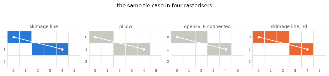
line and Pillow choose the same pixels. line_nd and OpenCV choose the same
pixels. Neither of our functions is unusual on this case — each has a peer.
Across every integer endpoint pair in a 9x9 box:
fns = {
    "sk.line": sk_line,
    "sk.line_nd": sk_nd,
    "pillow": pil_line,
    "opencv8": cv_line,
    "opencv4": lambda a, b: cv_line(a, b, 4),
}

drawn = {k: [f(a, b) for a, b in box] for k, f in fns.items()}
names = list(fns)
print(f"agreement over {len(box)} endpoint pairs")
print(f"{'':12}" + "".join(f"{n:>11}" for n in names))
for a in names:
    row = "".join(
        f"{sum(x == y for x, y in zip(drawn[a], drawn[b])) / len(box):>10.1%} "
        for b in names
    )
    print(f"{a:<12}{row}")
agreement over 6561 endpoint pairs
sk.line sk.line_nd pillow opencv8 opencv4
sk.line 100.0% 80.6% 100.0% 84.8% 21.0%
sk.line_nd 80.6% 100.0% 80.6% 80.6% 21.0%
pillow 100.0% 80.6% 100.0% 84.8% 21.0%
opencv8 84.8% 80.6% 84.8% 100.0% 21.0%
opencv4 21.0% 21.0% 21.0% 21.0% 100.0%
# Every eleventh pair: Pillow and OpenCV each build an image per call, so the
# full corpus is slow here. The skimage figures above use all 6561 pairs.
sample = box[::11]
print(f"{'':14}{'reversal':>12}{'translation':>14}")
for name, f in fns.items():
    print(
        f"{name:<14}{symmetry(f, sample, 'reversal'):>11.1%}"
        f"{symmetry(f, sample, 'translation'):>13.1%}"
    )
reversal translation
sk.line 68.7% 100.0%
sk.line_nd 100.0% 68.7%
pillow 68.7% 100.0%
opencv8 100.0% 100.0%
opencv4 100.0% 100.0%
What each library says it does
OpenCV states the algorithm in its own docstring: “For non-antialiased lines
with integer coordinates, the 8-connected or 4-connected Bresenham algorithm is
used. ... Antialiased lines are drawn using Gaussian filtering.” So both of its
non-antialiased line types are Bresenham, differing in
connectivity rather than in
method. Pillow’s
ImageDraw.line
documents no algorithm at all.
That leaves the question of how closely the three agree, which is measurable.
The correspondence is exact
Pillow draws the same pixels as skimage.draw.line, for the same endpoint
order. OpenCV draws the same pixels too, but for the endpoints ordered so that
the column index decreases — reversing a Bresenham line moves its
tie-breaking to the other side, and that reversal is the whole of the
difference.
def column_decreasing(a, b):
    """Order the endpoints so the column index decreases."""
    return (a, b) if b[1] <= a[1] else (b, a)


pillow_same = sum(pil_line(a, b) == sk_line(a, b) for a, b in box)
opencv_same = sum(cv_line(a, b) == sk_line(*column_decreasing(a, b)) for a, b in box)
print(f"over {len(box)} endpoint pairs")
print(f"   pillow  == sk.line, same endpoint order      : {pillow_same / len(box):.1%}")
print(f"   opencv8 == sk.line, column decreasing        : {opencv_same / len(box):.1%}")
over 6561 endpoint pairs
pillow == sk.line, same endpoint order : 100.0%
opencv8 == sk.line, column decreasing : 100.0%
Both are exact. So there is only one non-antialiased line algorithm across the three libraries; what differs is which end it starts from.
The rule is not obvious from the source, so it is worth showing how it was found. Take only the segments where our own line depends on direction, and ask which direction OpenCV matched:
from collections import Counter

pattern = Counter()
for a, b in box:
    if sk_line(a, b) == sk_line(b, a):
        continue                      # direction makes no difference here
    drawn_by_cv = cv_line(a, b)
    match = "forward" if drawn_by_cv == sk_line(a, b) else "reversed"
    d_col = b[1] - a[1]
    pattern[(match, "column increases" if d_col > 0 else "column decreases")] += 1

for (match, direction), n in sorted(pattern.items()):
    print(f"   opencv matched our {match:<8} run when the {direction}: {n:>5}")
opencv matched our forward run when the column decreases: 1000
opencv matched our reversed run when the column increases: 1000
The split is total: forward exactly when the column decreases. Neither the driving axis nor the row direction enters into it.
Anti-aliasing: the one place they genuinely differ
Every comparison so far has been between hard-edged lines. Softening the edges is a separate algorithm, and here the three libraries part company.
skimage.draw.line_aa implements the method of
Zingl (2012), an extension
of Bresenham that carries the error term into a coverage value. OpenCV’s
LINE_AA uses Gaussian filtering, by its own description. Pillow’s ImageDraw
has no anti-aliased line at all: it draws in two levels, and the usual advice
is to draw large and downsample.
from skimage.draw import line_aa

AA = 16
aa_start, aa_stop = (3, 2), (9, 13)

pillow_image = Image.new("L", (AA, AA), 0)
ImageDraw.Draw(pillow_image).line(
    [(aa_start[1], aa_start[0]), (aa_stop[1], aa_stop[0])], fill=255, width=1
)
pillow_aa = np.array(pillow_image) / 255

opencv_aa = np.zeros((AA, AA), np.uint8)
cv2.line(opencv_aa, (aa_start[1], aa_start[0]), (aa_stop[1], aa_stop[0]),
         255, 1, lineType=cv2.LINE_AA)
opencv_aa = opencv_aa / 255

skimage_aa = np.zeros((AA, AA))
rr, cc, value = line_aa(aa_start[0], aa_start[1], aa_stop[0], aa_stop[1])
skimage_aa[rr, cc] = value

for name, img in (("skimage line_aa", skimage_aa), ("opencv LINE_AA", opencv_aa),
                  ("pillow", pillow_aa)):
    print(f"{name:<18}{len(np.unique(img)):>3} distinct levels,"
          f"{int((img > 0).sum()):>4} pixels touched")
skimage line_aa 14 distinct levels, 26 pixels touched
opencv LINE_AA 25 distinct levels, 38 pixels touched
pillow 2 distinct levels, 12 pixels touched
Pillow reports two levels because it is not anti-aliasing at all. OpenCV
touches far more pixels than line_aa, which is what a Gaussian does: it
spreads coverage over a wider skirt than an error-term method.
fig, axes = plt.subplots(1, 3, figsize=(9.0, 2.8))
for ax, (name, img) in zip(axes, (("skimage line_aa", skimage_aa),
                                  ("opencv LINE_AA", opencv_aa),
                                  ("pillow, no anti-aliasing", pillow_aa))):
    ax.imshow(img, cmap=LinearSegmentedColormap.from_list("c", [C_OFF, C_LINE]),
              vmin=0, vmax=1, interpolation="nearest")
    ax.plot([aa_start[1], aa_stop[1]], [aa_start[0], aa_stop[0]],
            color=INK, linewidth=1.0)
    ax.set_xticks([])
    ax.set_yticks([])
    for spine in ax.spines.values():
        spine.set_visible(False)
    ax.set_title(name)
fig.suptitle("coverage, not just which pixels", y=1.04)
fig.tight_layout()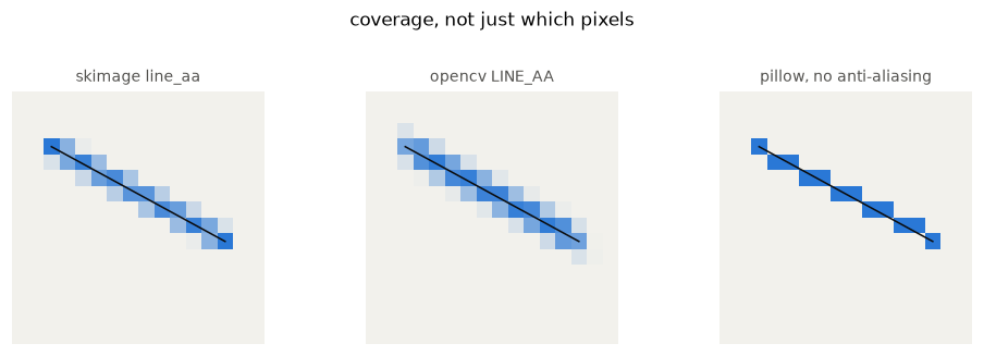
Two things fall out of those numbers.
skimage.draw.line is pixel-identical to Pillow, and OpenCV’s 8-connected
line equals our Bresenham run in one of the two endpoint orders in every
case — it is the same rasteriser with the endpoint order normalised first.
More importantly, OpenCV holds both symmetries at once. So the trade-off our two functions appear to make is not forced. Neither is at a local optimum.
OpenCV also offers a second rasteriser, chosen with lineType. It is a
different thing from the tie-breaking above, and it is the subject of the next
section.
8. The two connectivities
lineType selects between two rasterisers, cv2.LINE_8 and cv2.LINE_4.
They are not two settings of one algorithm. They draw different pixel sets,
with different guarantees, for different jobs.
import scipy.ndimage as ndi

# Slot 3 of the reference categorical palette; validates all-pairs with the
# blue and orange already in use.
C_FOUR = "#1baf7a"

S4 = np.array([[0, 1, 0], [1, 1, 1], [0, 1, 0]])
S8 = np.ones((3, 3), int)
What each one guarantees
An 8-connected line may step diagonally, so it needs one pixel per step of the longer axis. A 4-connected line may not, so it needs one pixel per step of both axes. That gives two exact formulas: a Chebyshev length and a Manhattan length, each plus one for the starting pixel.
c8 = c4 = 0
for a, b in box:
    di, dj = abs(a[0] - b[0]), abs(a[1] - b[1])
    c8 += len(cv_line(a, b, 8)) == max(di, dj) + 1
    c4 += len(cv_line(a, b, 4)) == di + dj + 1
print(f"over {len(box)} endpoint pairs")
print(f"   8-connected count == max(|di|, |dj|) + 1 : {c8 / len(box):.1%}")
print(f"   4-connected count == |di| + |dj| + 1     : {c4 / len(box):.1%}")
over 6561 endpoint pairs
8-connected count == max(|di|, |dj|) + 1 : 100.0%
4-connected count == |di| + |dj| + 1 : 100.0%
Both hold exactly, so lineType fixes how many pixels you get before any
rounding decision is taken.
a, b = (4, 4), (7, 13)
fig, axes = plt.subplots(1, 2, figsize=(7.2, 2.4))
for ax, conn, color, name in (
    (axes[0], 8, C_BOTH, "LINE_8, 8-connected"),
    (axes[1], 4, C_FOUR, "LINE_4, 4-connected"),
):
    pixel_axes(ax, (5, 12), f"{name}  ({len(cv_line(a, b, conn))} pixels)")
    fill(ax, {(i - 3, j - 3) for i, j in cv_line(a, b, conn)}, color)
    exact(ax, (a[0] - 3, a[1] - 3), (b[0] - 3, b[1] - 3), color="white")
fig.suptitle("the same segment, drawn twice", y=1.04)
fig.tight_layout()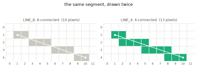
The difference is visible in the moves themselves. Walk each pixel set along the driving axis and look at the step taken between consecutive pixels:
def path_order(pixels, start, stop):
    """The pixels in the order the line visits them, major axis first."""
    delta = np.abs(np.subtract(stop, start))
    major = int(np.argmax(delta))
    minor = 1 - major
    sign = np.sign(np.subtract(stop, start))
    return sorted(pixels,
                  key=lambda ij: (sign[major] * ij[major], sign[minor] * ij[minor]))


def steps_taken(pixels, start, stop):
    """The distinct moves between consecutive pixels along the path."""
    walk = path_order(pixels, start, stop)
    return sorted({(abs(u[0] - v[0]), abs(u[1] - v[1]))
                   for u, v in zip(walk, walk[1:])})


for conn in (8, 4):
    pix = cv_line(a, b, conn)
    print(f"LINE_{conn}: {len(pix):>3} pixels, steps {steps_taken(pix, a, b)}")
LINE_8: 10 pixels, steps [(0, 1), (1, 1)]
LINE_4: 13 pixels, steps [(0, 1), (1, 0)]
One segment proves nothing, so check the whole corpus: no 4-connected line may contain a diagonal move.
diagonal_in_4 = sum((1, 1) in steps_taken(cv_line(u, v, 4), u, v) for u, v in box)
print(f"LINE_4 lines containing a (1, 1) move, out of {len(box)}: {diagonal_in_4}")
LINE_4 lines containing a (1, 1) move, out of 6561: 0
(1, 1) is a diagonal move. Only the 8-connected line makes one; the
4-connected line replaces each with a (1, 0) and a (0, 1), which is where
its extra pixels come from.
The pixel sets have different connectivity
The names describe a property of the drawn set, which is worth checking rather than assuming. Label each line as a binary image, once with a 4-connected structuring element and once with an 8-connected one. A line that is “4-connected” should be a single component under the 4-connected element.
def as_mask(pixels, shape=(CANVAS, CANVAS)):
    """The pixel set as a boolean image."""
    m = np.zeros(shape, bool)
    for i, j in pixels:
        m[i, j] = True
    return m


print(f"{'':10}{'one component under S4':>26}{'under S8':>12}")
for conn in (8, 4):
    n4 = sum(ndi.label(as_mask(cv_line(a, b, conn)), structure=S4)[1] == 1
             for a, b in box)
    n8 = sum(ndi.label(as_mask(cv_line(a, b, conn)), structure=S8)[1] == 1
             for a, b in box)
    print(f"LINE_{conn:<5}{n4 / len(box):>25.1%}{n8 / len(box):>12.1%}")

axis_aligned = sum(a[0] == b[0] or a[1] == b[1] for a, b in box)
print(f"\npairs with no diagonal step at all: {axis_aligned / len(box):>10.1%}")
one component under S4 under S8
LINE_8 21.0% 100.0%
LINE_4                       100.0%      100.0%

pairs with no diagonal step at all:      21.0%
An 8-connected line falls into separate pieces under 4-connectivity. The exceptions are exactly the axis-aligned segments, which take no diagonal step and so are 4-connected by accident — the two rates above agree to the digit. A 4-connected line holds together under both. That is the whole difference, stated as a property rather than as a name.
They are not nested
It is tempting to think the 4-connected line is the 8-connected one with corner pixels added. It is not.
nested = sum(cv_line(a, b, 8) <= cv_line(a, b, 4) for a, b in box)
print(f"8-connected set contained in the 4-connected set: {nested / len(box):.1%}")

example = next((a, b) for a, b in box if not cv_line(a, b, 8) <= cv_line(a, b, 4))
s8, s4 = cv_line(*example, 8), cv_line(*example, 4)
print(f"\nfirst counter-example: {example[0]} to {example[1]}")
print(f"   only in LINE_8: {sorted(s8 - s4)}")
print(f"   only in LINE_4: {sorted(s4 - s8)}")
8-connected set contained in the 4-connected set: 82.1%
first counter-example: (4, 4) to (5, 8)
only in LINE_8: [(4, 6)]
only in LINE_4: [(5, 5), (5, 6)]
a, b = example
lo = (min(a[0], b[0]) - 1, min(a[1], b[1]) - 1)
span = (abs(a[0] - b[0]) + 3, abs(a[1] - b[1]) + 3)
fig, axes = plt.subplots(1, 2, figsize=(7.2, 2.2))
for ax, pix, color, name in (
    (axes[0], s8, C_BOTH, "LINE_8"), (axes[1], s4, C_FOUR, "LINE_4")
):
    pixel_axes(ax, span, name)
    fill(ax, {(i - lo[0], j - lo[1]) for i, j in pix}, color)
    exact(ax, (a[0] - lo[0], a[1] - lo[1]), (b[0] - lo[0], b[1] - lo[1]),
          color="white")
fig.suptitle("neither set contains the other", y=1.06)
fig.tight_layout()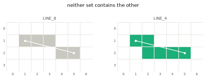
The two are independent rasterisations of the same segment, and neither is derived from the other. Each resolves awkward cases its own way. Which cases, and by what rule, is not something this notebook settles.
Why a 4-connected line exists: it seals
The reason to pay for the extra pixels is that a 4-connected curve is a barrier an 8-connected flood fill cannot cross. An 8-connected curve is not: a fill that may move diagonally slips between two diagonally adjacent pixels.
def barrier(conn, shape=(28, 40), a=(2, 0), b=(25, 39)):
    """Draw a line across the array, then label what it leaves free."""
    arr = np.zeros(shape, np.uint8)
    cv2.line(arr, (a[1], a[0]), (b[1], b[0]), 255, 1, lineType=conn)
    labels, n = ndi.label(~(arr > 0), structure=S8)
    return arr > 0, labels, n


for conn in (8, 4):
    _, _, n = barrier(conn)
    verdict = "sealed" if n > 1 else "the fill leaks through"
    print(f"LINE_{conn}: the free area is {n} component(s)  -> {verdict}")
LINE_8: the free area is 1 component(s) -> the fill leaks through
LINE_4: the free area is 2 component(s) -> sealed
fig, axes = plt.subplots(2, 1, figsize=(5.4, 4.6))
for ax, conn in zip(axes, (8, 4)):
    m, labels, n = barrier(conn)
    ax.imshow(np.where(m, 0, labels),
              cmap=ListedColormap([C_FOUR, C_OFF, C_LINE]), vmin=0, vmax=2)
    ax.set_xticks([])
    ax.set_yticks([])
    for spine in ax.spines.values():
        spine.set_visible(False)
    ax.set_title(f"LINE_{conn}: {n} free component(s)")
fig.legend(
    handles=[
        Patch(facecolor=C_FOUR, label="the line"),
        Patch(facecolor=C_OFF, label="one side"),
        Patch(facecolor=C_LINE, label="the other side"),
    ],
    loc="lower center", ncols=3, frameon=False, fontsize=8,
)
fig.suptitle("only the 4-connected line divides the array in two", y=1.0)
fig.tight_layout(rect=(0, 0.07, 1, 1))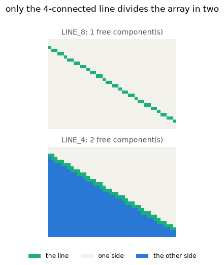
The top panel is a single region: the fill has walked through the line. The bottom panel is two. If you draw a boundary and then fill on one side of it, that is the whole ballgame, and it is why the option exists.
What scikit-image would need
skimage.draw has no 4-connected line, and line_nd’s “ndim-connected”
guarantee is the diagonal one. Closing the gap needs no new rasteriser: take
the Bresenham line and insert a corner pixel at each diagonal step, choosing
whichever of the two candidate corners lies nearer the true segment.
def line_4(start, stop):
    """Bresenham, with a corner pixel inserted at each diagonal step."""
    ii, jj = line(start[0], start[1], stop[0], stop[1])
    origin = np.asarray(start, float)
    direction = np.asarray(stop, float) - origin

    def offset(pixel):
        v = np.asarray(pixel, float) - origin
        return abs(v[0] * direction[1] - v[1] * direction[0])

    out = [(int(ii[0]), int(jj[0]))]
    for i, j in zip(ii[1:].tolist(), jj[1:].tolist()):
        pi, pj = out[-1]
        if i != pi and j != pj:
            out.append(min(((pi, j), (i, pj)), key=offset))
        out.append((i, j))
    return out
conn_ok = count_ok = 0
for a, b in box:
pix = line_4(a, b)
conn_ok += ndi.label(as_mask(pix), structure=S4)[1] == 1
count_ok += len(set(pix)) == abs(a[0] - b[0]) + abs(a[1] - b[1]) + 1
print(f"over {len(box)} endpoint pairs")
print(f" 4-connected {conn_ok / len(box):.1%}")
print(f" Manhattan pixel count {count_ok / len(box):.1%}")
arr = np.zeros((28, 40), np.uint8)
for i, j in line_4((2, 0), (25, 39)):
arr[i, j] = 255
print(f" seals the array {ndi.label(~(arr > 0), structure=S8)[1] > 1}")
same = sum(set(line_4(a, b)) == cv_line(a, b, 4) for a, b in box)
print(f" same pixels as LINE_4 {same / len(box):.1%}")over 6561 endpoint pairs
4-connected 100.0%
Manhattan pixel count 100.0%
seals the array True
same pixels as LINE_4 63.1%
It meets both guarantees and it seals. Where it differs from OpenCV, at the rate printed above, the difference is the corner chosen at each diagonal step — a tie-breaking question of exactly the kind the rest of this notebook is about, not a difference in what the two functions promise.
a, b = (4, 4), (7, 13)
fig, axes = plt.subplots(1, 2, figsize=(7.2, 2.4))
for ax, pix, color, name in (
    (axes[0], set(line_4(a, b)), C_ND, "candidate line_4"),
    (axes[1], cv_line(a, b, 4), C_FOUR, "opencv LINE_4"),
):
    pixel_axes(ax, (5, 12), name)
    fill(ax, {(i - 3, j - 3) for i, j in pix}, color)
    exact(ax, (a[0] - 3, a[1] - 3), (b[0] - 3, b[1] - 3), color="white")
fig.suptitle("same guarantees, different corners", y=1.04)
fig.tight_layout()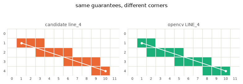
9. Bresenham in N dimensions, and what to call things
Bresenham is not a 2-D algorithm that happens to be popular. Wikipedia defines it as determining “the points of an n-dimensional raster”, and the 2-D case is the one everybody meets first. So the split in this notebook — Bresenham for two axes, a sampled line for N — is a fact about scikit-image, not about the algorithms.
The generalisation
The 2-D version of section 2 carries one error accumulator. The N-D version carries one per minor axis, and tests each independently. Nothing else changes.
def bresenham_nd(start, stop):
    """Bresenham in any number of dimensions: one error term per minor axis."""
    start, stop = np.array(start), np.array(stop)
    delta = np.abs(stop - start)
    step = np.sign(stop - start)

    major = int(np.argmax(delta))
    n_steps = int(delta[major])
    error = 2 * delta - n_steps          # one accumulator per axis

    at = start.copy()
    out = []
    for _ in range(n_steps):
        out.append(tuple(int(x) for x in at))
        for axis in range(len(delta)):
            if axis == major:
                continue
            if error[axis] >= 0:
                at[axis] += step[axis]
                error[axis] -= 2 * n_steps
            error[axis] += 2 * delta[axis]
        at[major] += step[major]

    out.append(tuple(int(x) for x in stop))
    return out
It has to reduce to the existing function when given two axes, or it is a different algorithm wearing the same name.
matches = sum(bresenham_nd(a, b) == sk_sequence(a, b) for a, b in all_pairs)
print(f"identical to skimage.draw.line in 2-D on {matches}/{len(all_pairs)} pairs"
      f"  ({matches / len(all_pairs):.1%})")
identical to skimage.draw.line in 2-D on 50625/50625 pairs (100.0%)
What it does in three dimensions
def nd_sequence(start, stop):
    """`line_nd` as a list of integer tuples, endpoint included."""
    return [tuple(int(x) for x in c)
            for c in zip(*line_nd(start, stop, endpoint=True))]


rng = np.random.default_rng(0)
grid = list(itertools.product(range(-4, 5), repeat=3))
choice = rng.choice(len(grid), size=(1500, 2))
triples = [(grid[a], grid[b]) for a, b in choice if grid[a] != grid[b]]

chebyshev = connected = 0
for start, stop in triples:
    pix = bresenham_nd(start, stop)
    chebyshev += len(pix) == max(abs(np.subtract(stop, start))) + 1
    connected += all(max(abs(np.subtract(v, u))) <= 1
                     for u, v in zip(pix, pix[1:]))

agree = sum(bresenham_nd(a, b) == nd_sequence(a, b) for a, b in triples)
print(f"over {len(triples)} random 3-D segments")
print(f"   point count is max(abs(delta)) + 1   : {chebyshev / len(triples):.1%}")
print(f"   every step moves at most 1 per axis  : {connected / len(triples):.1%}")
print(f"   identical to line_nd                 : {agree / len(triples):.1%}")
over 1499 random 3-D segments
point count is max(abs(delta)) + 1 : 100.0%
every step moves at most 1 per axis : 100.0%
identical to line_nd : 67.3%
The point count is the Chebyshev length again, and a step of at most one per axis means the line is 26-connected in 3-D — the direct generalisation of the diagonal connectivity of section 8.
The symmetries carry over unchanged, which is the useful part: the two algorithms hold the same complementary pair of properties in 3-D that they held in 2-D.
def holds(fn, kind, cases):
    ok = 0
    for start, stop in cases:
        if kind == "reversal":
            ok += set(fn(start, stop)) == set(fn(stop, start))
        else:
            shift = np.array([3, 1, 2])
            moved = {tuple(np.add(c, shift)) for c in fn(start, stop)}
            ok += moved == set(fn(tuple(np.add(start, shift)),
                                  tuple(np.add(stop, shift))))
    return ok / len(cases)


sample = triples[:600]
print(f"{'':16}{'reversal':>11}{'translation':>14}")
for name, fn in (("bresenham_nd", bresenham_nd), ("line_nd", nd_sequence)):
    print(f"{name:<16}{holds(fn, 'reversal', sample):>10.1%}"
          f"{holds(fn, 'translation', sample):>14.1%}")
reversal translation
bresenham_nd 56.7% 100.0%
line_nd 100.0% 62.2%
A 3-D scatter is hard to read, so project the line onto the two planes that contain the major axis. The staircases are then as legible as in section 4. Projection can send two different 3-D positions to one cell, so the grey shows agreement in the projection; the exact disagreements are listed below it.
# All three axes vary, and the two algorithms disagree on part of the run.
start3, stop3 = (0, 0, 0), (2, 4, 8)
walks = {"bresenham_nd": bresenham_nd(start3, stop3),
         "line_nd": nd_sequence(start3, stop3)}

fig, axes = plt.subplots(2, 2, figsize=(8.4, 4.0))
for row, (name, walk) in enumerate(walks.items()):
    colour = C_LINE if name == "bresenham_nd" else C_ND
    for col, axis in enumerate((0, 1)):
        ax = axes[row, col]
        shared = {(v[axis], v[2]) for v in walks["bresenham_nd"]} & \
                 {(v[axis], v[2]) for v in walks["line_nd"]}
        mine = {(v[axis], v[2]) for v in walk}
        pixel_axes(ax, (5 if axis else 3, 9),
                   f"{name}, axis {axis} against axis 2")
        fill(ax, shared, C_BOTH)
        fill(ax, mine - shared, colour)
        exact(ax, (start3[axis], start3[2]), (stop3[axis], stop3[2]),
              color="white")
fig.suptitle("grey where the projections coincide, coloured where they do not", y=1.02)
fig.tight_layout()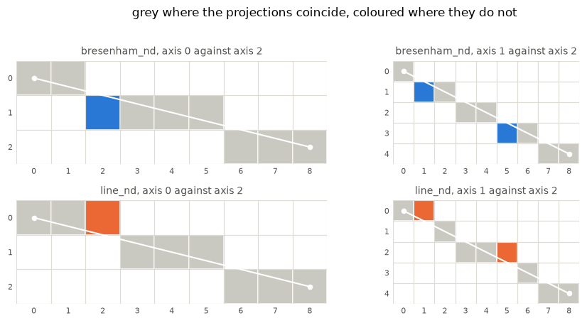
differ = [(u, v) for u, v in zip(walks["bresenham_nd"], walks["line_nd"]) if u != v]
print(f"{len(differ)} of {len(walks['bresenham_nd'])} positions differ:")
for u, v in differ:
    print(f"   bresenham_nd {u}   line_nd {v}")
3 of 9 positions differ:
bresenham_nd (0, 1, 1) line_nd (0, 0, 1)
bresenham_nd (1, 1, 2) line_nd (0, 1, 2)
bresenham_nd (1, 3, 5) line_nd (1, 2, 5)
Elsewhere
ITK’s BresenhamLine
is templated over dimension, and is the closest thing to a reference N-D
implementation in an imaging library. Alois Zingl’s published
plotLine3d is the
common ancestor of several 3-D-only ports (see bresenham_nd_cython.md’s
mechanism-A discussion). OpenCV and Pillow are 2-D only.
One warning about the literature: “3-D Bresenham” names two different
things. Some implementations use integer error terms, as above. Others set
step = delta / max(delta) and accumulate in floating point, which is a
digital differential analyser with Bresenham’s name attached — and that is what
line_nd is.
The naming is the problem
skimage.draw has three line functions, and they are distinguished along three
different axes:
| Name | What the suffix means |
|---|---|
line | nothing; it is the default |
line_aa | a property of the output: anti-aliased |
line_nd | a dimensionality |
None of them names an algorithm, and the one that looks like a dimensionality
claim is really an algorithm claim: line_nd differs from line in 2-D as
well, on about a fifth of segments, as section 5 measured.
Decision D1 of the port makes this sharper. Once line takes coordinate
tuples, line(start, stop) and line_nd(start, stop) have identical
signatures. If line also became N-D, the two would be interchangeable at
every call site while returning different pixels for a third of 3-D segments.
What actually separates them
Not the dimensionality, and for a user not really the algorithm either, but the guarantees:
line (Bresenham) | line_nd (sampled) | |
|---|---|---|
| Endpoints | integers only | floats accepted |
| Endpoint included | always | endpoint= |
| Output | integer indices | integers, or floats with integer=False |
| Arithmetic | exact integer | floating point |
| Translation invariant | yes | no |
| Reversal symmetric | no | yes, for integer endpoints |
The float endpoints are not a convenience that Bresenham could absorb. Integer arithmetic needs integer deltas, so a float segment has to be rounded first, and that is a different line:
print("line_nd on the true float segment:")
print("  ", nd_sequence((0.4, 0.2), (3.6, 9.8)))
print("bresenham on the rounded endpoints:")
print("  ", bresenham_nd((0, 0), (4, 10)))
line_nd on the true float segment:
[(0, 0), (1, 1), (1, 2), (1, 3), (2, 4), (2, 5), (2, 6), (3, 7), (3, 8), (3, 9), (4, 10)]
bresenham on the rounded endpoints:
[(0, 0), (0, 1), (1, 2), (1, 3), (2, 4), (2, 5), (2, 6), (3, 7), (3, 8), (4, 9), (4, 10)]
Refactoring options
Each of these is a real choice, and none is free.
A. Extend line to N-D, leave line_nd alone.
For: the smallest change; Bresenham becomes available in 3-D where ITK users
already expect it.
Against: the names then actively mislead. line_nd would no longer be the
N-D one, and nothing in either name would say which algorithm you get. This is
the worst option for a reader coming to the API fresh.
B. One function with a method= keyword.
line(start, stop, method="bresenham") or method="dda".
For: one entry point; the choice is visible at the call site; new methods
(supercover, 4-connected) slot in later.
Against: the methods do not accept the same arguments. endpoint and float
coordinates are meaningless for Bresenham, so the signature grows parameters
that are valid only for some values of method — the pattern that made
warp’s inverse_map hard to document.
C. Rename line_nd to line_dda, and extend line to N-D.
For: both names then say what they are, and the dimensionality stops being
part of anybody’s name because both work in N-D. The distinction on offer is
the real one.
Against: dda is jargon; a user who does not know the term learns nothing
from it. It also breaks every existing line_nd call.
D. One N-D Bresenham, drop the sampled version.
For: one line function, one set of guarantees, no choice to explain.
Against: it deletes float endpoints, endpoint=False and integer=False,
which the cell above shows cannot be recovered by rounding. Multi-point path
drawing depends on endpoint=False. Not viable as it stands.
E. Name by the guarantee, not the algorithm.
Something like line for the exact-integer one and line_sampled for the
other.
For: names the thing the user chooses on. A caller who needs float endpoints
reads “sampled” and knows; “dda” tells them nothing.
Against: invents vocabulary that no other library uses, so it helps nobody
arriving from ITK or the graphics literature.
F. Leave the names, document the difference.
For: no breakage; the cost is one paragraph in each docstring and a
See Also.
Against: leaves two functions with identical signatures and different results
distinguished by a suffix that describes neither difference. Section 5 shows
people would have to read carefully to find out which they want.
A recommendation, with the caveat that it is a judgement and not a
measurement. C, with E’s reasoning applied to the docstrings: extend line
to N dimensions, rename line_nd to line_dda, keep line_nd as a
deprecated alias, and open each docstring with the guarantee rather than the
algorithm — “exact integer arithmetic, integer endpoints” against “samples the
segment, accepts float endpoints”. That gives honest names for the people who
know the algorithms, and a first sentence that decides it for the people who do
not.
Option B is the tempting one and worth resisting for the reason warp teaches:
a keyword that changes which other keywords are legal is a worse interface than
two functions.
10. Two ways forward
Fix 1: round half up in line_nd
Half-to-even makes the drawn shape depend on the parity of an absolute coordinate. Nothing wants that.
Rounding half up has a pedigree here, not just a property. Section 3 quoted
Knuth stepping around the tie by an “infinitesimal shift of the path”. Half-up
is that shift, written down: floor(x + 1/2) is the limit of
round(x + e) as e falls to zero from above, so every tie resolves as if the
path had been nudged by a hair in one fixed direction. Half-to-even is not the
limit of any shift, because which way a tie goes depends on the parity of the
neighbouring integer rather than on the path — which is the same fact as its
failure of translation invariance, seen from the other side.
The objection on the record. When this was proposed during review of
#2043,
Juan Nunez-Iglesias answered that np.floor makes evenly spaced samples come
out unevenly spaced, where np.round does not:
spaced = np.array([0.5, 1.25, 2.0, 2.75, 3.5])   # the example from the PR
for name, rule in (("np.round", np.round),
                   ("np.floor", np.floor),
                   ("floor(x) + 0.5, as written in the PR",
                    lambda a: np.floor(a) + 0.5),
                   ("floor(x + 0.5), half up", lambda a: np.floor(a + 0.5))):
    got = rule(spaced).astype(int)
    print(f"   {name:<38}{str(got):<18}steps {np.diff(got)}")
np.round [0 1 2 3 4] steps [1 1 1 1]
np.floor [0 1 2 2 3] steps [1 1 0 1]
floor(x) + 0.5, as written in the PR [0 1 2 2 3] steps [1 1 0 1]
floor(x + 0.5), half up [1 1 2 3 4] steps [0 1 1 1]
Two things are true at once. The expression tested in the review,
(np.floor(coords0) + 0.5).astype(int), is not half-up rounding — astype(int)
truncates, so it returns plain np.floor. Half-up is np.floor(x + 0.5), and
it was never evaluated.
But the objection partly survives evaluation anyway. Half-up gives
[1, 1, 2, 3, 4], with a repeat, where np.round gives [0, 1, 2, 3, 4] with
none. So for this spacing np.round really does produce the tidier sequence.
What settles it is that the repeat is not a defect. Section 2 showed a shallow line advancing along its major axis while the minor axis stands still; repeats on a minor axis are what a shallow line is. A gap is a different kind of event: it breaks the line. The two are not comparable costs, and only one of them is a correctness failure.
def line_nd_halfup_pixels(a, b):
    """Ordered pixels from `line_nd` with half-up rounding."""
    a, b = np.asarray(a, float), np.asarray(b, float)
    npoints = int(np.ceil(np.max(np.abs(b - a)))) + 1
    coords = np.floor(np.linspace(a, b, npoints, endpoint=True).T + 0.5).astype(int)
    return [tuple(int(v) for v in c) for c in coords.T]


print("the PR's spacing, drawn as an actual line")
for a, b in (((0.5, 0.0), (3.5, 4.0)), ((0, 0), (3, 4))):
    now = nd_pixels(a, b)
    up = line_nd_halfup_pixels(a, b)
    hop = lambda pix: [int(np.max(np.abs(np.subtract(y, x))))
                       for x, y in zip(pix, pix[1:])]
    print(f"   {a} -> {b}")
    print(f"      line_nd now   {now}  steps {hop(now)}")
    print(f"      half up       {up}  steps {hop(up)}")
the PR's spacing, drawn as an actual line
(0.5, 0.0) -> (3.5, 4.0)
line_nd now [(0, 0), (1, 1), (2, 2), (3, 3), (4, 4)] steps [1, 1, 1, 1]
half up [(1, 0), (1, 1), (2, 2), (3, 3), (4, 4)] steps [1, 1, 1, 1]
(0, 0) -> (3, 4)
line_nd now [(0, 0), (1, 1), (2, 2), (2, 3), (3, 4)] steps [1, 1, 1, 1]
half up [(0, 0), (1, 1), (2, 2), (2, 3), (3, 4)] steps [1, 1, 1, 1]
Both are 8-connected, both have the same length, and they differ in which pixel stands for the tie. The uneven spacing the review worried about does not reach the drawn line.
_round_safe is not a partial fix for the parity problem, and it is worth being
precise about what it is. Half-to-even has two distinct consequences, and
the guard addresses one of them while leaving the other alone.
The first is a gap. line_nd samples at most one pixel apart, so rounding
must not put two consecutive samples two pixels apart. Half-to-even can:
np.round([0.5, 1.5]) is [0, 2]. The guard aims at exactly that, and on an
ascending axis it hits: a gap needs two consecutive samples on exact halves,
which needs a half fraction and unit spacing, which is what the guard tests.
On a descending axis it misses, for the signed-1 reason section 3 sets out,
and the line comes apart.
The second is the parity dependence itself: at a tie, which way the rounding goes depends on whether the neighbouring integer is even, so the drawn shape depends on where the line sits rather than on its direction. That produces no gap, so the guard never sees it.
Rounding half up removes both at once, and in both directions, which is why the guard becomes unnecessary rather than merely redundant. That it cannot gap is provable, not just observed.
Write f(x) = floor(x + 1/2). Two facts bound its error:
f(x) <= x + 1/2, sincefloor(y) <= y. Equality holds exactly whenx + 1/2is whole, that is whenxlies on a half.f(x) > x - 1/2, sincefloor(y) > y - 1. This one is strict.
So the rounding error f(x) - x lies in the half-open interval
(-1/2, +1/2]. It reaches +1/2, and approaches -1/2 without ever
attaining it.
Now take two samples no more than one apart, with the second the larger. Applying the upper bound to one term and the strict lower bound to the other:
    f(x[k+1]) - f(x[k])  <  (x[k+1] + 1/2) - (x[k] - 1/2)
                         =  (x[k+1] - x[k]) + 1  <=  2
The left side is an integer strictly less than 2, so it is at most 1, and f
is non-decreasing so it is at least 0. Reversing the roles covers the other
direction. Hence
| f(x[k+1]) - f(x[k]) | <= 1for any two samples at most one apart. No gap is possible — for any offset, any
spacing, and without needing the samples to be equidistant, so the proof is
slightly stronger than the assumption _round_safe documents.
Where the argument fails for the other rules. Everything turns on that one
strict inequality. np.round attains both ends of [-1/2, +1/2]: its error
is -1/2 at 0.5 and +1/2 at 1.5. With equalities on both sides the bound
becomes exactly 2, and 2 is then reachable — np.round([0.5, 1.5]) is [0, 2].
That makes it a statement about half-openness rather than about banker’s
rounding in particular, which is a falsifiable prediction: rounding halves away
from zero also attains both ends, at -0.5 and +0.5, so it should gap too —
at the origin, where those two meet.
rules = {
    "half-up": lambda x: np.floor(x + 0.5),
    "half-to-even": np.round,
    "half-away": lambda x: np.sign(x) * np.floor(np.abs(x) + 0.5),
}

fine = np.arange(-4, 4, 1 / 512)
print(f"{'rule':<14}{'error range':>22}{'worst jump, step 1':>22}")
for name, rule in rules.items():
    errors = rule(fine) - fine
    steps = np.arange(-4, 4, 0.25)
    jump = max(abs(float(rule(np.float64(a + 1.0)) - rule(np.float64(a))))
               for a in steps)
    print(f"{name:<14}[{errors.min():+.3f}, {errors.max():+.3f}]{jump:>21.0f}")
rule error range worst jump, step 1
half-up [-0.498, +0.500] 1
half-to-even [-0.500, +0.500] 2
half-away [-0.500, +0.500] 2
Half-up never produces a negative error at all on a grid of halves, and its
minimum over a fine grid approaches -1/2 without reaching it. The other two
touch both ends, and both gap.
So the guard addresses the gap alone, and only on axes that count up. A
one-word repair — abs(coords[1] - coords[0]) == 1 — would finish that job,
and would still leave the exact float equalities, the inspect-only-the-first-
coordinate assumption, and the parity dependence in place. Fix 1 retires all
four together.
Rounding half up is translation-invariant by construction, because
floor(x + t + 0.5) == floor(x + 0.5) + t for whole t.
def line_nd_halfup(a, b):
    """`line_nd` with half-up rounding instead of half-to-even."""
    a, b = np.asarray(a, float), np.asarray(b, float)
    npoints = int(np.ceil(np.max(np.abs(b - a)))) + 1
    coords = np.floor(np.linspace(a, b, npoints, endpoint=True).T + 0.5).astype(int)
    return set(zip(*(c.tolist() for c in coords)))


fig, axes = plt.subplots(2, 4, figsize=(9.6, 4.0))
for col, t in enumerate(range(4)):
    a, b = (t, 0), (1 + t, 4)
    for row, (f, name) in enumerate(
        ((sk_nd, "line_nd, now"), (line_nd_halfup, "line_nd, half up"))
    ):
        ax = axes[row, col]
        pixel_axes(ax, (6, 6), f"{name} (+{t})")
        fill(ax, f(a, b), C_ND)
        exact(ax, a, b, color="white")
fig.suptitle("half-up rounding makes line_nd keep its shape when it moves", y=1.01)
fig.tight_layout()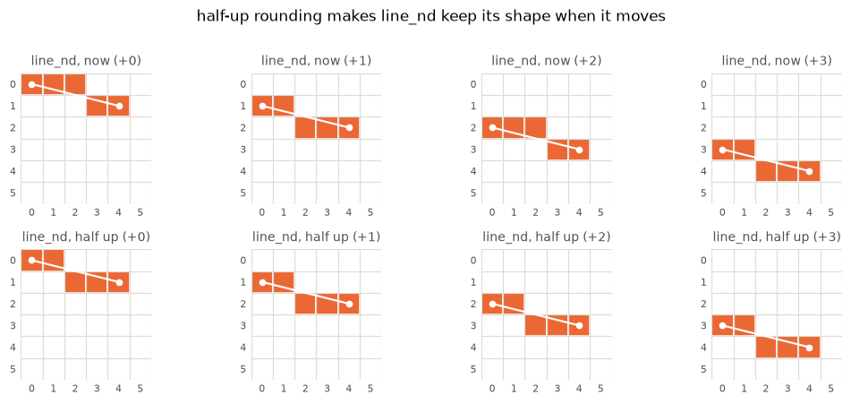
Fix 2: normalise the endpoint order in line
Knuth ends his note with a requirement on the renderer, not on the caller. If two halves of a bisected angle are to look alike, he writes, the bisecting line must be one about which “reflections ... always map pixels into pixels”, and “furthermore, your line-rendering algorithm should produce symmetrical results about the line of reflection” — with a citation to Bresenham’s ambiguities paper. A renderer that changes its answer when the ends are swapped does not produce symmetrical results, so it cannot meet that condition.
Sorting the two endpoints before rasterising makes the result independent of
which end was named first. Any rule that depends only on the unordered pair
works; OpenCV uses a different one from sorted, and matching it exactly is
not a requirement.
def line_sorted(a, b):
    """`line` with the endpoint order normalised."""
    a, b = sorted([tuple(a), tuple(b)])
    return sk_line(a, b)


fig, axes = plt.subplots(1, 4, figsize=(9.6, 2.1))
panels = [
    (sk_line, p, q, "line, forward"),
    (sk_line, q, p, "line, backward"),
    (line_sorted, p, q, "sorted, forward"),
    (line_sorted, q, p, "sorted, backward"),
]
for ax, (f, a, b, name) in zip(axes, panels):
    pixel_axes(ax, shape, name)
    fill(ax, f(a, b), C_LINE)
    exact(ax, a, b, color="white")
fig.suptitle("normalising the endpoints makes line direction-independent", y=1.04)
fig.tight_layout()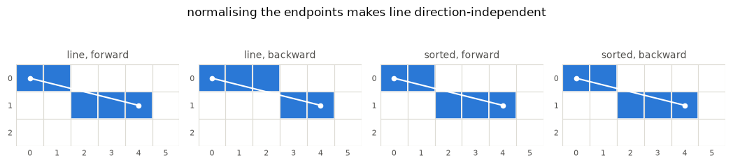
What each fix costs
changed_nd = sum(sk_nd(a, b) != line_nd_halfup(a, b) for a, b in box)
changed_ln = sum(sk_line(a, b) != line_sorted(a, b) for a, b in box)
agree_now = sum(sk_line(a, b) == sk_nd(a, b) for a, b in box)
agree_fix = sum(line_sorted(a, b) == line_nd_halfup(a, b) for a, b in box)
n_box = len(box)

print(f"line_nd output changes under half-up rounding : {changed_nd / n_box:6.1%}")
print(f"line output changes under sorted endpoints    : {changed_ln / n_box:6.1%}")
print(f"line and line_nd agree, now                   : {agree_now / n_box:6.1%}")
print(f"line and line_nd agree, both fixed            : {agree_fix / n_box:6.1%}")

for name, f in (("line, sorted", line_sorted), ("line_nd, half up", line_nd_halfup)):
    print(
        f"\n{name}: reversal {symmetry(f, box, 'reversal'):.1%},"
        f" translation {symmetry(f, box, 'translation'):.1%}"
    )
line_nd output changes under half-up rounding : 19.4%
line output changes under sorted endpoints : 15.2%
line and line_nd agree, now : 80.6%
line and line_nd agree, both fixed : 92.4%
line, sorted: reversal 100.0%, translation 100.0%
line_nd, half up: reversal 100.0%, translation 100.0%
Both fixes reach 100% on both symmetries, matching OpenCV’s guarantees.
The case for fix 1 is strong: parity-dependent rasterisation is a defect, and no comparator library has it. The case for fix 2 is weaker — the current behaviour is textbook Bresenham and matches Pillow exactly — but a drawing function whose output depends on which end you named first is surprising, and the change is one line.
Both change results, so both belong in skimage2 with a migration note, not
in a patch release.
11. What review already knew
Both defects in this notebook were raised before line_nd was merged, and the
literature naming them is older still.
line_nd arrived in
#2043, opened in April
2016 and merged in September 2019. The rounding question is in the opening post:
half-to-even “would result in broken lines”, and the guard is proposed as the
remedy in the same paragraph. It went in as written.
At the moment of merge Stéfan van der Walt recorded two reservations (comment): “my concern with the rounding function used here, and also that we have not properly explored existing N-d line drawing methods”. Sections 3 and 10 are the first of those; section 9 is the second. The reply was that the API was now fixed and improvements were welcome as later pull requests (comment), and none followed.
The same thread also asks the question section 9 arrives at from the other
direction. Mark Harfouche asked whether line should be deprecated in favour of
line_nd
(comment),
and was told it need not be settled there. Section 9 concludes it should not be:
they are different algorithms with different guarantees, and the naming is what
needs fixing rather than the count of functions.
The two papers Stéfan linked in that thread are the ones cited above.
Bresenham (1987) is the source
for section 6: equal-error ties let the chosen pixels “differ depending on the
direction it is drawn”.
Knuth (1990) supplies the digitisation rule
line_nd implements, the explicit statement that it is undefined on a tie, and
the closing requirement that a renderer be symmetric.
Knuth’s actual theorem is about something this notebook does not cover, and it
is worth knowing where the boundary is. He proves that when a line of slope
a/b meets one of slope c/d, the junction takes one of exactly |ad - bc|
distinct digital shapes as the meeting point moves, each equally likely. That is
a statement about joins, not about single segments: it says a polyline’s
corners will not all look alike however good the line renderer is. No choice of
rounding rule removes it.
12. What not to do
Do not try to make line and line_nd agree. Even with both fixes they still
differ on a small fraction of segments, and that residue is inherent: an exact
integer error term and a sampled-then-rounded line pick different pixels at
ties. They are different algorithms with different guarantees, and both are
worth keeping.
resid = [(a, b) for a, b in box if line_sorted(a, b) != line_nd_halfup(a, b)]
a, b = resid[0]
lo = (min(a[0], b[0]) - 1, min(a[1], b[1]) - 1)

fig, axes = plt.subplots(1, 2, figsize=(7.2, 2.4))
span = (abs(a[0] - b[0]) + 3, abs(a[1] - b[1]) + 3)
for ax, (f, color, name) in zip(
    axes,
    ((line_sorted, C_LINE, "line, sorted"), (line_nd_halfup, C_ND, "line_nd, half up")),
):
    pixel_axes(ax, span, name)
    fill(ax, {(i - lo[0], j - lo[1]) for i, j in f(a, b)}, color)
    exact(ax, (a[0] - lo[0], a[1] - lo[1]), (b[0] - lo[0], b[1] - lo[1]), color="white")
fig.suptitle(f"both fixed, still different: {a} to {b}", y=1.04)
fig.tight_layout()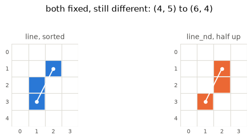
Summary
line | line_nd | Pillow | OpenCV | |
|---|---|---|---|---|
| Algorithm | integer Bresenham | sample, then round per axis | integer Bresenham | Bresenham, ends normalised |
| Dimensions | 2 | N | 2 | 2 |
| Input | integer only | float or integer | integer | integer (sub-pixel via shift) |
| Stop point | always included | excluded unless endpoint=True | included | included |
| Connectivity | diagonal | diagonal | diagonal | diagonal or 4-connected |
| Reversal symmetric | no | yes, for integer endpoints | no | yes |
| Translation invariant | yes | no | yes | yes |
One non-antialiased 8-connected algorithm underlies skimage.draw.line, Pillow,
and OpenCV’s LINE_8. skimage.draw.line and Pillow agree pixel for pixel;
OpenCV’s LINE_8 agrees too, for the endpoints ordered so the column
decreases. The differences in the table are tie-breaking and endpoint order,
not method. OpenCV’s LINE_4 is a second rasteriser, covered in section 8.
Anti-aliasing is where they actually diverge, and section 7 measures that:
line_aa follows Zingl, OpenCV filters with a Gaussian and touches a wider
skirt, and Pillow does not anti-alias lines at all.
Measured over integer endpoints only, for segments up to about twelve pixels
long, against the comparator versions this build actually used. line_aa is
compared only for coverage, not for the endpoint treatment it would want
alongside line.
import PIL
import skimage

print(f"scikit-image {skimage.__version__}")
print(f"Pillow       {PIL.__version__}")
print(f"OpenCV       {cv2.__version__}")
scikit-image 0.26.1rc0.dev0
Pillow 12.3.0
OpenCV 5.0.0