PR 8074 adds a fifth
ridge filter, from Jerman et al.
(2016). on_frangi.md and
on_meijering.md catalogue defects in two of the four already there, so the
question for a new one is whether it repeats them.
It avoids Frangi’s polarity and sigma-order defects. It shares Meijering’s non-locality, which comes from the published rule rather than from the port. The missing is inert for this ratio-only response at ordinary amplitudes; an absolute eigenvalue tolerance makes that claim conditional. The rest of the notebook measures those points and sketches candidate follow-ups for the author.
Coordinates are in array order.
import numpy as np
import pandas as pd
import matplotlib.pyplot as plt
from matplotlib.colors import LinearSegmentedColormap

from nbhelper import show_table
import skimage as ski
from skimage.feature import hessian_matrix, hessian_matrix_eigvals
from skimage.filters import sato, frangi, meijeringfatal: not a git repository (or any of the parent directories): .git
fatal: not a git repository (or any of the parent directories): .git
# Slots 1 to 3 of the reference categorical palette, validated all-pairs;
# same palette as the other notebooks here.
C_ONE, C_TWO, C_THREE = "#2a78d6", "#eb6834", "#1baf7a"
INK, MUTED, GRID = "#0b0b0b", "#52514e", "#dedcd5"
SEQ = LinearSegmentedColormap.from_list("seq", ["#f7f7f4", C_ONE])

plt.rcParams.update(
    {"figure.dpi": 110, "font.size": 9, "axes.titlesize": 9,
     "axes.titlecolor": MUTED, "figure.facecolor": "white"}
)


def bare(ax, title=None):
    ax.set_xticks([]); ax.set_yticks([])
    for spine in ax.spines.values():
        spine.set_visible(False)
    if title:
        ax.set_title(title)
    return ax


def recede(ax, title=None):
    ax.tick_params(labelsize=8, colors=MUTED)
    for spine in ("top", "right"):
        ax.spines[spine].set_visible(False)
    for spine in ("left", "bottom"):
        ax.spines[spine].set_color(GRID)
    if title:
        ax.set_title(title)
    return ax
1. What the filter computes¶
Sort the Hessian eigenvalues by magnitude, . Jerman’s measure uses the largest one and a regularised version of it, , which replaces small values by a floor set at a fraction of the largest at that scale over the image (their equation 13):
The response is then equations 14 and 15:
and the filter takes the maximum over a list of σ. In 2-D the paper introduces an auxiliary eigenvalue by setting . This is the 2-D specialization of a 3-D model with a circular cross-section; an elliptical cross-section is therefore outside that equivalence.
The PR implements this response for 2-D and 3-D images. skimage.filters.jerman
is not in this notebook’s environment, so the version below is an executable
transcription, with a power argument added for section 3. The default path is
the PR as checked out. relative_tol=True is a notebook-only candidate fix.
def jerman_core(image, sigmas, tau=0.75, black_ridges=True, mode="reflect",
                power=0.0, relative_tol=False):
    """Transcribe PR 8074, with optional notebook-only variants.

    `power=0` is the PR as written; `power=2` adds the `c = sigma.^2` scaling
    that Jerman's own MATLAB applies. `relative_tol=True` applies a candidate
    relative floor (`eps * max(λ₃⁺)` here — illustrative, not a proposed
    constant) and is not in the PR. Returns the fused maximum and the
    per-scale responses.
    """
    image = image.astype(float, copy=False)
    if not black_ridges:
        image = -image
    fused, per_scale = np.zeros_like(image), {}
    for sigma in sigmas:
        eigvals = hessian_matrix_eigvals(
            hessian_matrix(image, sigma, mode=mode, use_gaussian_derivatives=True))
        eigvals = np.take_along_axis(eigvals, abs(eigvals).argsort(0), 0)
        eigvals = eigvals * sigma**power

        if relative_tol:
            if image.ndim == 2:
                lambda2_raw = eigvals[1]
                lambda3_raw = lambda2_raw
            else:
                lambda2_raw, lambda3_raw = eigvals[1:]

            lambda3_max = np.maximum(lambda3_raw, 0).max()
            tol = np.finfo(image.dtype).eps * lambda3_max
            lambda2 = np.maximum(lambda2_raw, tol)
            lambda3 = np.maximum(lambda3_raw, tol)
            floor = tau * lambda3_max
            rho = np.full_like(lambda3, floor)
            rho[lambda3_raw <= 0] = 0
            rho[lambda3_raw > floor] = lambda3_raw[lambda3_raw > floor]
        else:
            tol = 1e-10
            if image.ndim == 2:
                (lambda2,) = np.maximum(eigvals[1:], tol)
                lambda3 = lambda2.copy()
            else:
                lambda2, lambda3 = np.maximum(eigvals[1:], tol)

            floor = tau * lambda3.max()                # eq. 13
            rho = np.full_like(lambda3, floor)
            rho[lambda3 <= tol] = 0
            rho[lambda3 > floor] = lambda3[lambda3 > floor]

        numerator = lambda2**2 * (rho - lambda2) * 27
        denominator = (lambda2 + rho) ** 3
        if relative_tol:
            vals = np.divide(
                numerator,
                denominator,
                out=np.zeros_like(numerator),
                where=denominator != 0,
            )                                                               # eq. 14
        else:
            vals = numerator / denominator                                  # eq. 14
        vals[(lambda2 >= rho / 2) & (rho > tol)] = 1                       # eq. 15
        vals[(lambda2 <= tol) | (rho <= tol)] = 0
        per_scale[sigma] = vals
        fused = np.maximum(fused, vals)
    return fused, per_scale
PHOTO = ski.util.img_as_float(ski.data.camera())[::2, ::2]
LOCALITY_PHOTO = np.tile(PHOTO, (2, 2))
SIGMAS = (1, 3, 5, 7, 9)
N = 241
rows, cols = np.indices((N, N), dtype=float)
MID = N // 2
FIXTURE_2D = np.array([
[4.0, 4.0, 0.0, 0.0, 4.0, 4.0],
[4.0, 4.0, 0.0, 0.0, 4.0, 4.0],
[0.0, 0.0, 0.0, 0.0, 0.0, 0.0],
[0.0, 0.0, 0.0, 0.0, 0.0, 0.0],
[4.0, 4.0, 0.0, 0.0, 4.0, 4.0],
[4.0, 4.0, 0.0, 0.0, 4.0, 4.0],
])
FIXTURE_2D_EXPECTED = np.array([
[0.0, 0.0, 1.0, 1.0, 0.0, 0.0],
[0.0, 0.0, 1.0, 1.0, 0.0, 0.0],
[1.0, 1.0, 1.0, 1.0, 1.0, 1.0],
[1.0, 1.0, 1.0, 1.0, 1.0, 1.0],
[0.0, 0.0, 1.0, 1.0, 0.0, 0.0],
[0.0, 0.0, 1.0, 1.0, 0.0, 0.0],
])
z3, y3, x3 = np.indices((17, 17, 17), dtype=float)
VOLUME3D = 1 - (
np.exp(-((x3 - 8) ** 2 + (y3 - 8) ** 2) / (2 * 2**2))
* (1 + 0.2 * np.cos(z3 / 3))
)The following checks are executable. The 2-D fixture is the small response example used in the PR discussion. The 3-D volume varies along all three axes, so it exercises the distinct 3-D eigenvalue branch. The amplitude comparison shows the original PR result before and after the candidate tolerance change.
fixture_out, _ = jerman_core(FIXTURE_2D, [1])
volume_out, _ = jerman_core(VOLUME3D, [1])
volume_scaled, _ = jerman_core(1e-6 * VOLUME3D, [1])
volume_relative, _ = jerman_core(VOLUME3D, [1], relative_tol=True)
volume_relative_scaled, _ = jerman_core(
    1e-6 * VOLUME3D, [1], relative_tol=True
)

assert np.array_equal(fixture_out, FIXTURE_2D_EXPECTED)
assert volume_out.shape == VOLUME3D.shape
assert np.isfinite(volume_out).all()
assert ((0 <= volume_out) & (volume_out <= 1)).all()
assert volume_out[8, 8, 8] > 0.9
assert np.allclose(volume_relative_scaled, volume_relative)
print("2-D fixture passed")
print(f"original PR, 3-D amplitude change: "
      f"{np.abs(volume_scaled - volume_out).max():.2e}")
print(f"candidate relative tolerance: "
      f"{np.abs(volume_relative_scaled - volume_relative).max():.2e}")
2-D fixture passed
original PR, 3-D amplitude change: 9.44e-16
candidate relative tolerance: 9.44e-16
2. What the PR changes against the reference¶
The PR’s docstring says it “was written based on the MATLAB implementation by Tim Jerman”. Against the paper, equations 13, 14 and 15 are transcribed correctly, including the substitution that section B prescribes for 2-D, the three-way rule, and the 27 that is 33 from . The PR’s comments cite the equation numbers and they are the right ones.
One detail in the paper has no counterpart in the PR, and it is not only a detail of the reference implementation but the definition of the Hessian itself. Equation 1 is
where is the Gaussian standard deviation, and with the built in.
Jerman’s MATLAB implements it as
c = sigma.^2; Hxx = c*Hxx; .... That is Lindeberg’s scale normalisation. Its
absence is related to on_frangi.md’s D2: on ideal ridges, the unnormalized
structuredness term cannot select a finite width, and it is the subject of the
still-open issue
#7711. Finding it
missing here looks like the same bug arriving in a new filter.
The missing factor is not a defect in this response. The paper says why.
The MATLAB code is not otherwise a numerical oracle for this PR. Its
vesselness2D.m
and
vesselness3D.m
code smooths with a Gaussian, uses finite differences with replicate
boundaries, casts the input to single, removes small eigenvalues, normalizes
the fused response by its global maximum, and zeros responses below 10-2.
The PR uses Gaussian derivatives through
hessian_matrix, accepts the caller’s mode and cval, preserves the
supported floating-point precision, and does not apply that final normalization
or threshold. The linked source is useful for checking the equations, but a
fixture generated from it will not match the PR unless these stages are
specified separately.
3. Why the missing σ² changes nothing¶
Look at what the response depends on. Every branch of equations 14 and 15 is a function of and only through their ratio: dividing numerator and denominator of the third branch by gives
and the two other branches are comparisons — is — which are ratio tests too. Now is either or , and both are linear in the Hessian. So multiplying the Hessian by any positive constant, included, leaves and therefore unchanged apart from floating-point roundoff. This is the equation-level statement; the implementation also depends on the boundary value and floating-point dtype.
without = jerman_core(-PHOTO, SIGMAS, power=0.0)[0]
with_sigma2 = jerman_core(-PHOTO, SIGMAS, power=2.0)[0]

rows_scale = [{"comparison": "no σ power vs σ² on the Hessian",
               "max |difference|": f"{np.abs(without - with_sigma2).max():.2e}",
               "pixels differing at all": f"{(without != with_sigma2).mean():.1%}"}]
for factor in (3.0, 100.0):
    scaled = jerman_core(-PHOTO * factor, SIGMAS)[0]
    rows_scale.append({"comparison": f"image × {factor:g} vs image × 1",
                       "max |difference|": f"{np.abs(scaled - without).max():.2e}",
                       "pixels differing at all": f"{(scaled != without).mean():.1%}"})
show_table(pd.DataFrame(rows_scale), index="comparison")The differences are at roundoff level. Scaling the whole image gives the same result to numerical precision. The filter is invariant to positive Hessian rescaling, so equation 1’s is inert for this enhancement function and the PR loses nothing by dropping it.
“For this enhancement function” is the necessary qualifier. Equation 1 is the
paper’s general Hessian, shared with the six established functions it compares
against — Frangi’s, Sato’s, Li’s, Erdt’s, Zhou’s and plain — and
those are not ratios, so they need the exactly as sato does. It is
redundant only in the one function the PR implements.
The paper states the property directly in its discussion, as a design feature rather than an accident:
The main benefit of the ratio of eigenvalue magnitudes is that it effectively cancels the magnitude decays towards a structure’s periphery. It also normalizes the response across different scales and thus exhibits a similar response on structures of different sizes.
This corrects on_meijering.md §5.4, which lists the PR as dropping “the
σ² its own reference applies” and warns that merging it would give
scikit-image “a third ridge filter with D2”. The first half is true and the
second is wrong: D2 is about scale normalization for an implicit scale
comparison, and σ² is not the only way to make this response comparable across
scales. The next section measures what the supplied scale list does.
3.1 Candidate fix: make the tolerance relative¶
The PR uses eigval_tol = 1e-10 as an absolute floor. The clipping and the two
special cases in equation 15 therefore introduce an input-unit threshold. The
candidate path scales the floor by the largest positive at each
scale. Here that factor is machine epsilon — enough to show that some
relative floor restores amplitude invariance in this probe, but sharper than a
production suggestion. A PR change would more likely use a small multiple of
eps (or of lambda3_max itself), chosen against float32 inputs and near-null
Hessians, not eps alone.
reference = jerman_core(-PHOTO, SIGMAS)[0]
reference_relative = jerman_core(-PHOTO, SIGMAS, relative_tol=True)[0]

rows_amp = []
for amplitude in (1e2, 1.0, 1e-2, 1e-4, 1e-5, 1e-6):
    scaled = jerman_core(-PHOTO * amplitude, SIGMAS)[0]
    scaled_relative = jerman_core(
        -PHOTO * amplitude, SIGMAS, relative_tol=True
    )[0]
    without = jerman_core(-PHOTO * amplitude, SIGMAS, power=0.0)[0]
    with_s2 = jerman_core(-PHOTO * amplitude, SIGMAS, power=2.0)[0]
    without_relative = jerman_core(
        -PHOTO * amplitude, SIGMAS, power=0.0, relative_tol=True
    )[0]
    with_s2_relative = jerman_core(
        -PHOTO * amplitude, SIGMAS, power=2.0, relative_tol=True
    )[0]
    rows_amp.append({
        "image ×": f"{amplitude:.0e}",
        "original vs amplitude 1": f"{np.abs(scaled - reference).max():.1e}",
        "candidate vs amplitude 1":
            f"{np.abs(scaled_relative - reference_relative).max():.1e}",
        "original no σ power vs σ²":
            f"{np.abs(without - with_s2).max():.1e}",
        "candidate no σ power vs σ²":
            f"{np.abs(without_relative - with_s2_relative).max():.1e}",
    })
show_table(pd.DataFrame(rows_amp), index="image ×")The original PR changes when the image amplitude crosses its absolute floor.
The candidate relative floor keeps both the amplitude comparison and the
sigma**2 comparison at floating-point scale in this probe. That supports the
direction of the fix, not the exact eps multiplier. This check uses
mode="reflect"; a nonzero cval is not rescaled when the image is rescaled
and is a separate boundary condition. A relative-tolerance change of this kind
could be proposed for the author’s PR, with the constant chosen separately.
3.2 An inherited cost the PR does not control¶
One more thing follows the filter in from hessian_matrix rather than from the
PR, and it is worth knowing because jerman’s own default triggers it.
_hessian_matrix_with_gaussian chooses
truncate = 8 if all(s > 1 for s in sigma) else 100so any scale at or below σ = 1 uses truncate=100 in each derivative pass
instead of 8. The helper passes σ/ to gaussian_filter, and the
Hessian applies two such passes. The documented default
sigmas=range(1, 10, 2) starts at exactly 1.
import scipy.ndimage as ndi_spy

calls = []
_real_gaussian = ndi_spy.gaussian_filter


def _spy(inp, sigma, **kwargs):
    calls.append((round(float(np.atleast_1d(sigma)[0]), 4), kwargs.get("truncate")))
    return _real_gaussian(inp, sigma, **kwargs)


ndi_spy.gaussian_filter = _spy
try:
    jerman_core(-PHOTO, range(1, 10, 2))
finally:
    ndi_spy.gaussian_filter = _real_gaussian

show_table(pd.DataFrame(
    [{"scaled σ passed to gaussian_filter": s, "truncate": t,
      "kernel radius (px)": int(t * s + 0.5)}
for s, t in sorted(set(calls))]))The finest scale uses a 71-pixel radius per Gaussian call where the next one up
uses 17. on_hessian.md measures what that buys: nothing detectable — the kernel
moments are bit-identical to the truncate=8 ones and the output difference is
at floating-point roundoff. It is an inherited cost, not a defect introduced here,
and it is not in the PR’s diff at all — but a reviewer timing the new filter
against the others should know that its default sigmas puts it on the
expensive branch and the others’ defaults do too.
4. Scale-uniform response, not a scale estimator¶
The invariance of section 3 has a consequence worth stating carefully, because the obvious reading of it is wrong.
Scale normalization usually exists so that responses at different σ can be
compared, and the winning scale can estimate structure size. sato
multiplies by , meijering should multiply by
(on_meijering.md §5), and frangi has no such factor. jerman uses a ratio
and returns only the maximum response. It does not return the scale that won,
and it has no explicit scale estimator.
The paper says that its aim is “a similar response on structures of different sizes”. This describes uniformity across scale, not a promise that the supplied scales cannot change the output. At a scale that satisfies the saturation condition, that scale returns exactly 1. Other scales can remain below 1, so a tie at the saturated value occurs only when the relevant scales all saturate.
What is left to measure is the unsaturated regime, which the paper’s own regularisation exists to handle, and there σ does change the answer: through which structures are tubular at that scale, and through the image-wide maximum that sets . Both push one way.
SIGMA_GRID = (1, 2, 3, 4, 6, 8, 10, 12)
# A dominant narrow ridge sets the per-scale floor. The weaker ridges remain
# unsaturated, so their implicit winning scales can be compared.
scene = -(3.0 * np.exp(-((cols - 20) ** 2) / (2 * 1.5**2))
          + 0.30 * np.exp(-((cols - 80) ** 2) / (2 * 2.0**2))
          + 0.30 * np.exp(-((cols - 140) ** 2) / (2 * 6.0**2))
          + 0.30 * np.exp(-((cols - 200) ** 2) / (2 * 10.0**2)))
_, per = jerman_core(scene, SIGMA_GRID)

rows_pick = []
for column, width in ((80, 2.0), (140, 6.0), (200, 10.0)):
    values = {s: per[s][MID, column] for s in SIGMA_GRID}
    rows_pick.append({"true width": width,
                      "winning σ": max(values, key=values.get),
                      **{f"σ={s}": round(values[s], 3) for s in SIGMA_GRID}})
show_table(pd.DataFrame(rows_pick), index="true width")In this construction, three ridges of quite different width and equal contrast are all won by the coarsest σ on offer. The response rises monotonically with σ in each row; extend the list and the winner moves with it.
This is not a general proof that Jerman always favors coarse scales. It shows
that the fused maximum is not a calibrated width estimator and that the useful
range of sigmas can be bounded by the scene and the global regularizer, not
only by structure width. A caller choosing smin and smax, which the paper
says should follow “the respective minimal and maximal expected size of the
structures of interest”, gets no warning from the filter if they overshoot.
The same distinction applies to frangi: a finest-scale preference can occur
in its ridge construction, but no single scale is guaranteed to win for every
image. The two filters should not be described as mirror-image scale failures.
fig, ax = plt.subplots(figsize=(6.2, 3.0))
for (column, width), colour in zip(((80, 2.0), (140, 6.0), (200, 10.0)),
                                   (C_ONE, C_TWO, C_THREE)):
    ax.plot(SIGMA_GRID, [per[s][MID, column] for s in SIGMA_GRID], "o-", color=colour,
            lw=1.7, ms=4, label=f"ridge of width {width:g}")
recede(ax, "response against σ: no interior maximum for any width")
ax.set_xlabel("σ", fontsize=8, color=MUTED)
ax.set_ylabel("response", fontsize=8, color=MUTED)
ax.legend(frameon=False, fontsize=8)
fig.tight_layout()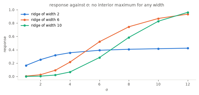
5. τ·max(λ₃) is a per-scale global statistic¶
The floor in equation 13 is a fraction of the largest over the
whole image, recomputed at every scale. Structurally that is the defect
on_meijering.md is about — a whole-image number inside the scale loop — and
here it is deliberate, with both halves of the choice stated in the paper. Why
a regulariser at all:
In image regions of uniform intensity, however, all eigenvalue magnitudes are low and the ratio is ill-behaved. This problem has been addressed by regularizing the eigenvalue with the highest magnitude to a fraction τ of the overall highest magnitude.
and why per scale:
To normalize the response of proposed enhancement function across the scales, is computed for each scale separately.
So the global maximum is the price of making a ratio well behaved where both its terms vanish, and the per-scale recomputation supplies the paper’s separate scale-normalization step. It is not mathematically equivalent to . Neither is a transcription error. What the paper does not discuss is the consequence: the response at a pixel now depends on pixels arbitrarily far away.
def far_field(fn, image, spot=(0, 0), value=10.0, keep=160):
    """Relative change beyond `keep` pixels when one pixel is brightened."""
    edited = image.copy()
    edited[spot] = value
    before, after = fn(image), fn(edited)
    far = (slice(keep, None), slice(keep, None))
    return (np.abs(before[far] - after[far]).max()
            / max(np.abs(before[far]).max(), 1e-12))


def crop_change(fn, image, size=400, margin=110):
    """Change in the shared interior when the surroundings are cropped away."""
    whole, part = fn(image)[:size, :size], fn(image[:size, :size])
    inner = (slice(margin, -margin),) * 2
    return (np.abs(whole[inner] - part[inner]).max()
            / max(np.abs(whole[inner]).max(), 1e-12))


probes = {}
for label, fn in (
        ("jerman (PR 8074)", lambda im: jerman_core(im, SIGMAS)[0]),
        ("meijering", lambda im: meijering(im, sigmas=SIGMAS)),
        ("frangi", lambda im: frangi(im, sigmas=SIGMAS)),
        ("sato", lambda im: sato(im, sigmas=SIGMAS, mode="reflect"))):
    probes[label] = {
        "one distant pixel": f"{far_field(fn, LOCALITY_PHOTO, keep=160):.2%}",
        "crop the surroundings":
            f"{crop_change(fn, LOCALITY_PHOTO):.2%}",
    }
show_table(pd.DataFrame(probes).T)The probe margins exceed the approximate two-pass support of the largest scale,
so they do not measure ordinary convolution spillover. sato is local, while
the other three also use image-wide statistics. jerman joins them. The
mechanism is direct enough to watch: hold a ridge fixed and brighten something
far away from it.
probe_ridge = np.exp(-((cols - 120) ** 2) / (2 * 4.0**2))

rows_far = []
for amplitude in (0.0, 4.0, 8.0, 16.0, 40.0):
    scene_far = probe_ridge + (
        amplitude * np.exp(-((rows - 30) ** 2 + (cols - 30) ** 2) / (2 * 3.0**2))
        if amplitude else 0.0)
    _, per_far = jerman_core(-scene_far, [4.0])
    eigvals = hessian_matrix_eigvals(
        hessian_matrix(-scene_far, 4.0, mode="reflect",
                       use_gaussian_derivatives=True))
    eigvals = np.take_along_axis(eigvals, abs(eigvals).argsort(0), 0)
    rows_far.append({
        "distant bar amplitude": amplitude,
        "τ·max(λ₃)": round(0.75 * np.maximum(eigvals[1], 0).max(), 5),
        "response at the untouched ridge": round(per_far[4.0][MID, 120], 6)})
show_table(pd.DataFrame(rows_far), index="distant bar amplitude")The local Hessian at the ridge does not change. Its score falls from 1.0 to
under 0.06 because something in the far corner raises the image-wide maximum.
That is the same failure on_meijering.md documents for meijering, arriving
through a different formula.
Unlike frangi, though, the statistic is recomputed at every scale rather than
frozen at the first, so the ordering defect of on_frangi.md D3 does not
appear here.
ascending = jerman_core(-PHOTO, SIGMAS)[0]
descending = jerman_core(-PHOTO, SIGMAS[::-1])[0]
print(f"jerman, max |ascending sigmas − descending| = "
      f"{np.abs(ascending - descending).max():.1e}")
print(f"frangi, the same comparison                = "
      f"{np.abs(frangi(PHOTO, sigmas=SIGMAS) - frangi(PHOTO, sigmas=SIGMAS[::-1])).max():.1e}")
jerman, max |ascending sigmas − descending| = 0.0e+00
frangi, the same comparison = 1.0e+00
6. What the PR gets right¶
Two things it would have been easy to get wrong.
Wrong-polarity rejection works. frangi clips the eigenvalue denominator
to 1e-10 and relies on the ratio exploding, which fails when the numerator is
also zero — on_frangi.md D1, where black_ridges becomes inert on an ideal
ridge. jerman clips with the absolute tolerance in the PR, then tests the
clipped values explicitly and sets those pixels to zero. The relative version
is the candidate from §3.1. The test catches the pixels the clip created.
bright_ridge = np.exp(-((cols - MID) ** 2) / (2 * 3.0**2))

show_table(pd.DataFrame(
    [{"filter": "jerman (PR 8074)",
      "black_ridges=True": jerman_core(bright_ridge, [3.0])[0][MID, MID],
      "black_ridges=False":
          jerman_core(bright_ridge, [3.0], black_ridges=False)[0][MID, MID]},
     {"filter": "frangi",
      "black_ridges=True": frangi(bright_ridge, sigmas=[3.0])[MID, MID],
      "black_ridges=False":
          frangi(bright_ridge, sigmas=[3.0], black_ridges=False)[MID, MID]}]
).round(6), index="filter")A bright ridge scored as a dark one reads exactly zero under jerman and the
filter’s maximum under frangi. Note that the probe is the ridge centre: a
bright bar has genuinely dark-valley-like shoulders, so the image maximum is
non-zero for both filters and would not show this.
The response is bounded. Equation 15 caps it at 1 by construction, so the output needs no normalisation. The fused maximum is order-independent, which is why the ordering check above comes out exactly zero.
fused = jerman_core(-PHOTO, SIGMAS)[0]
print(f"camera, output range: [{fused.min():.4f}, {fused.max():.4f}]")
print(f"fraction saturated at exactly 1.0: {(fused == 1.0).mean():.2%}")
camera, output range: [0.0000, 1.0000]
fraction saturated at exactly 1.0: 14.75%
That cap has a cost worth naming. When all relevant scales saturate, the fused response is a tie at exactly 1 and the filter reports no scale at all. A single saturating scale can also hide lower responses at the other scales. Section 4 uses an unsaturated construction to measure the scale dependence.
7. Side by side¶
Default black_ridges=True (dark vessels on a bright field) — the opposite of
the -PHOTO / -scene probes above, which flip polarity so a bright ridge is
scored as a dark one. retina needs no flip.
fig, axes = plt.subplots(1, 4, figsize=(11.5, 3.0))
retina = ski.util.img_as_float(ski.color.rgb2gray(ski.data.retina()))[::4, ::4]
for ax, (name, out) in zip(axes, (
        ("input", retina),
        ("jerman (PR 8074)", jerman_core(retina, SIGMAS)[0]),
        ("frangi", frangi(retina, sigmas=SIGMAS)),
        ("sato", sato(retina, sigmas=SIGMAS, mode="reflect")))):
    bare(ax, name)
    ax.imshow(out, cmap="gray" if name == "input" else SEQ)
fig.suptitle("the dark vessels of `retina`, default parameters", y=1.03)
fig.tight_layout()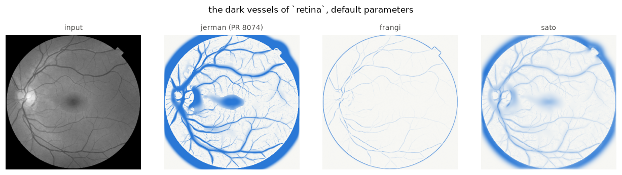
8. The tests the PR adds¶
jerman is added to the existing parametrised cases — null matrix, energy
decrease, linearity, black/white equivalence, dtype, and border management —
and one algorithm-specific test,
test_jerman_result_decrease_with_tau_increase. That test uses five tau values
from 0 to 2 and derives and
for .
The inherited linearity tests use constant arrays, so their Hessians are zero and they do not test amplitude behavior. The fixture, 3-D volume, amplitude sweep, and tau-policy table below are notebook checks, not tests added by the PR.
What is not covered follows from the sections above:
| property | tested? |
|---|---|
| τ monotonicity | yes, with a derivation; the PR test uses 0 to 2 |
| known 2-D response | measured here, not in the PR |
| genuine 3-D branch | measured here, not in the PR |
| amplitude invariance | original PR fails at small amplitudes; candidate passes this probe |
| tau guidance | paper recommends 0.5–1; PR accepts outside that; own τ test uses 0–2 |
| agreement with Jerman’s MATLAB output | no |
behaviour across sigmas | no |
| locality — does a distant pixel change the answer? | measured here, not in a unit test |
| bounded output | yes, on the 3-D fixture; saturation rate is not a unit-test contract |
The paper describes tau as a cutoff between zero and one, evaluates it over
that interval, and recommends 0.5 to 1 for the reported trade-off between
uniformity and false positives. The PR documents that recommendation but still
accepts values outside it — including the 0 and 2 used by
test_jerman_result_decrease_with_tau_increase. Hard-rejecting anything
outside would therefore conflict with a test the PR already ships.
A docstring note (or a warning) fits the paper’s guidance without breaking that
sweep; a hard interval would need the monotonicity test narrowed first.
def checked_jerman(image, sigmas, tau, *, hard=False):
    """Illustrate soft vs hard handling of the recommended tau interval."""
    if not 0.5 <= tau <= 1:
        msg = "`tau` is usually between 0.5 and 1."
        if hard:
            raise ValueError(msg)
        # Soft path: document only. Callers still get a response.
    return jerman_core(image, sigmas, tau=tau)[0]


tau_rows = []
for tau in (0.25, 0.75, 1.25):
    tau_rows.append({
        "tau": tau,
        "PR / soft guidance": "accepted",
        "hard reject [0.5, 1]": (
            "rejected" if not 0.5 <= tau <= 1 else "accepted"
        ),
    })
show_table(pd.DataFrame(tau_rows), index="tau")
# Keep the soft path exercised so the wrapper is not dead code.
assert checked_jerman(PHOTO, [3], 0.25, hard=False).shape == PHOTO.shapeThe MATLAB output is not a direct fixture target because its Hessian and postprocessing differ from the PR. The equation-level fixture is the stable regression target; a separate MATLAB comparison must compare intermediate stages or reproduce the MATLAB conventions. The fixture and relative-tolerance checks are suggestions for the author’s PR; the tau table is a policy choice, not a drop-in validation patch.
9. Summary¶
| finding | verdict | evidence |
|---|---|---|
| faithful transcription of equations 13–15 | yes, at the equation level | §1 fixture and executable transcription |
| drops equation 1’s | immaterial at ordinary amplitudes for this ratio-only response | §3, original and candidate comparisons |
| tolerance scale | original PR is absolute; relative floor restores invariance here (eps is illustrative) | §3.1, amplitude sweep |
| scale estimator | none explicit; supplied scales can still change the fused response | §4 |
| locality | fails, through — from the paper, not the port | §5, support-separated probes |
depends on the order of sigmas | no | §5 |
| wrong-polarity rejection | correct, unlike frangi | §6 |
| bounded output | yes, with possible scale ties | §6 |
The recommendation is narrow. The PR implements equations 13 to 15, and the
missing of equation 1 is inert for this ratio-only response at ordinary
amplitudes. The absolute tolerance makes that statement conditional; a
relative eigenvalue floor is worth suggesting to the author, with the
multiplier chosen more carefully than the eps used in §3.1. The MATLAB
implementation remains a different numerical pipeline, so the PR should state
that it ports the response equations rather than reproducing MATLAB output.
The non-locality comes from the published algorithm rather than from the port,
and meijering has shipped with the same property for years. The tau floor
couples every pixel to the largest positive in the frame, so
cropping the image can change the answer. A docstring sentence on that coupling,
and on the usual 0.5–1 range for tau without hard-rejecting the PR’s
existing 0–2 sweep, could be proposed for the author’s PR.
Limits. One 2-D photograph, one retina crop, and synthetic Gaussian ridges,
at mode='reflect' and tau=0.75 unless stated. The 3-D check uses one
non-separable synthetic volume and one scale. The locality probes use a tiled
camera image and margins chosen to exceed the estimated two-pass support.
The notebook does not import the PR worktree, and it does not compare output
with MATLAB. The MATLAB discussion in §2 is based on reading the published
source, not on executing it.
print(f"scikit-image {ski.__version__}")scikit-image 0.26.1rc0.dev0
- Jerman, T., Pernus, F., Likar, B., & Spiclin, Z. (2016). Enhancement of Vascular Structures in 3D and 2D Angiographic Images. IEEE Transactions on Medical Imaging, 35(9), 2107–2118. 10.1109/tmi.2016.2550102