On the blob detectors

skimage.feature offers three blob detectors — blob_dog, blob_log and blob_doh — with matching signatures and a shared output format. They are presented as three routes to one answer, differing in speed.

They differ in more than speed. Measured against discs of known radius, one is accurate to a few per cent, one reports radii a quarter too small, and one reports them up to a third too large. This notebook explains where each difference comes from, and which are defects rather than documented approximations.

Coordinates are in array order throughout: the first index runs down the picture, the second runs right.

import time

import numpy as np
import scipy.ndimage as ndi
import matplotlib.pyplot as plt
from matplotlib.colors import LinearSegmentedColormap

import skimage as ski
from skimage.feature import blob_dog, blob_log, blob_doh, hessian_matrix_det

fatal: not a git repository (or any of the parent directories): .git
fatal: not a git repository (or any of the parent directories): .git

# Comparator.
import cv2

# Slots 1 to 3 of the reference categorical palette, validated all-pairs.
C_ONE = "#2a78d6"
C_TWO = "#eb6834"
C_THREE = "#1baf7a"
INK, MUTED, GRID = "#0b0b0b", "#52514e", "#dedcd5"
SEQ = LinearSegmentedColormap.from_list("seq", ["#f7f7f4", C_ONE])

plt.rcParams.update(
    {"figure.dpi": 110, "font.size": 9, "axes.titlesize": 9,
     "axes.titlecolor": MUTED, "figure.facecolor": "white"}
)


def bare(ax, title=None):
    """Strip an axis down to the data."""
    ax.set_xticks([])
    ax.set_yticks([])
    for spine in ax.spines.values():
        spine.set_visible(False)
    if title is not None:
        ax.set_title(title)
    return ax


def recede(ax, title=None):
    """Keep the ticks, but make the frame recede."""
    ax.tick_params(labelsize=8, colors=MUTED)
    for spine in ("top", "right"):
        ax.spines[spine].set_visible(False)
    for spine in ("left", "bottom"):
        ax.spines[spine].set_color(GRID)
    if title is not None:
        ax.set_title(title)
    return ax

1. A test image with known answers¶

Four discs, well separated, with radii spanning the useful range.

N = 400
rows, cols = np.indices((N, N))
TRUTH = [(80, 80, 6), (80, 220, 10), (220, 80, 16), (220, 260, 24)]

discs = np.zeros((N, N))
for r0, c0, radius in TRUTH:
    discs[(rows - r0) ** 2 + (cols - c0) ** 2 <= radius**2] = 1.0

fig, ax = plt.subplots(figsize=(3.2, 3.2))
bare(ax, "four discs, radii 6, 10, 16 and 24")
ax.imshow(discs, cmap="gray")
fig.tight_layout()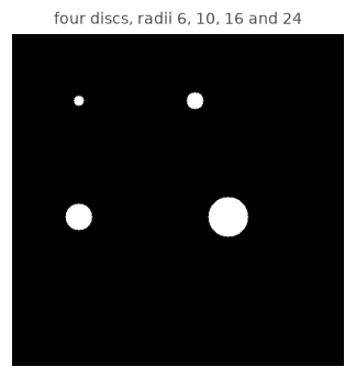

2. What a blob detector does¶

Each detector builds a scale-normalised response — a filter applied at many scales, scaled so that responses at different scales are comparable — and then looks for maxima in the three-dimensional stack of position and scale. The position of a maximum gives the blob’s centre, and its scale gives the size.

That normalisation is the whole trick. A plain second derivative gets smaller as sigma grows, so without it the smallest scale always wins. Multiplying by the right power of sigma cancels that, and the power differs by filter: sigma**2 for a Laplacian, sigma**4 for a Hessian determinant.

The three detectors differ in which filter they use.

	filter	documented radius
`blob_log`	Laplacian of Gaussian, `sigma*2 div(grad(G)) * f`	`sqrt(2) * sigma`
`blob_dog`	difference of two Gaussians, approximating the above	`sqrt(2) * sigma`
`blob_doh`	determinant of the Hessian, by box filters	`sigma`

The radius conventions really do differ, and they are documented that way. Every comparison below uses each detector’s own convention, taken from its docstring.

CONVENTION = {"blob_dog": np.sqrt(2), "blob_log": np.sqrt(2), "blob_doh": 1.0}

3. What each one reports¶

found = {
    "blob_dog": blob_dog(discs, min_sigma=2, max_sigma=30, threshold=0.05),
    "blob_log": blob_log(discs, min_sigma=2, max_sigma=30, num_sigma=30,
                         threshold=0.05),
    "blob_doh": blob_doh(discs, min_sigma=2, max_sigma=30, num_sigma=30,
                         threshold=0.005),
}


def matched(name, r0, c0, window=400):
    """The detection nearest a known centre, as a radius in pixels."""
    near = [b for b in found[name] if (b[0] - r0) ** 2 + (b[1] - c0) ** 2 < window]
    if not near:
        return np.nan
    best = min(near, key=lambda b: (b[0] - r0) ** 2 + (b[1] - c0) ** 2)
    return best[2] * CONVENTION[name]


print(f"{'true radius':>12}" + "".join(f"{n:>22}" for n in found))
for r0, c0, radius in TRUTH:
    line = f"{radius:>12}"
    for name in found:
        got = matched(name, r0, c0)
        line += f"{got:>13.1f} ({(got - radius) / radius:+.0%})"
    print(line)
print()
print("blobs found, against four present:",
      {n: len(b) for n, b in found.items()})

 true radius              blob_dog              blob_log              blob_doh
           6          4.5 (-25%)          5.6 (-7%)          7.8 (+30%)
          10          7.2 (-28%)          9.7 (-3%)         11.7 (+17%)
          16         11.6 (-28%)         16.5 (+3%)         21.3 (+33%)
          24         18.5 (-23%)         23.3 (-3%)         25.2 (+5%)

blobs found, against four present: {'blob_dog': 4, 'blob_log': 4, 'blob_doh': 4}

fig, axes = plt.subplots(1, 3, figsize=(9.6, 3.4))
for ax, (name, blobs) in zip(axes, found.items()):
    bare(ax, name)
    ax.imshow(discs, cmap="gray")
    for r0, c0, radius in TRUTH:
        ax.add_patch(plt.Circle((c0, r0), radius, fill=False, color=C_THREE,
                                lw=1.2, ls=":"))
    for b in blobs:
        ax.add_patch(plt.Circle((b[1], b[0]), b[2] * CONVENTION[name],
                                fill=False, color=C_TWO, lw=1.4))
fig.suptitle("dotted green: the true disc.   orange: what the detector reports",
             y=1.03)
fig.tight_layout()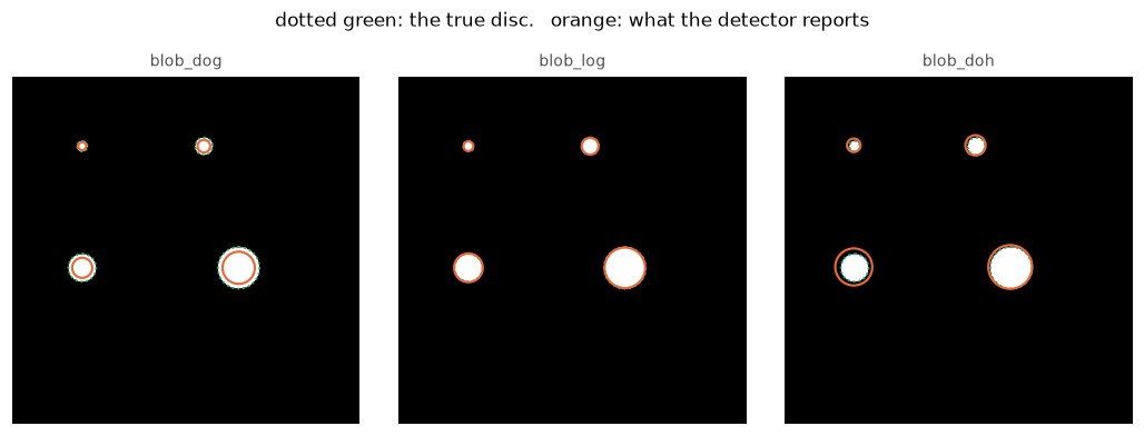

blob_log traces the discs closely. blob_dog sits consistently inside them and blob_doh consistently outside. Neither of those is noise: both biases are systematic and repeat at every radius.

4. `blob_dog`: a documented approximation¶

The difference of two Gaussians at sigma and k * sigma approximates the scale-normalised Laplacian, and the approximation improves as k approaches 1. blob_dog reports the smaller of the pair, so the reported sigma sits below the scale the response actually peaked at.

print(f"{'sigma_ratio k':>15}{'reported radius for the r=16 disc':>36}")
for ratio in (1.6, 1.4, 1.2, 1.1, 1.05):
    got = blob_dog(discs, min_sigma=2, max_sigma=30, sigma_ratio=ratio,
                   threshold=0.05)
    near = [b for b in got if (b[0] - 220) ** 2 + (b[1] - 80) ** 2 < 400]
    radius = near[0][2] * np.sqrt(2) if near else np.nan
    print(f"{ratio:>15}{radius:>25.1f} ({(radius - 16) / 16:+.0%})")

  sigma_ratio k   reported radius for the r=16 disc
            1.6                     11.6 (-28%)

            1.4                     15.2 (-5%)

            1.2                     14.6 (-9%)

            1.1                     15.7 (-2%)

           1.05                     15.6 (-2%)

The bias falls from -28% at the default to about -2%, which identifies it: it is the sigma_ratio approximation, behaving as the theory says it should. It is not monotone in k, because changing sigma_ratio also changes which discrete scales get computed. sigma_ratio defaults to 1.6, the value Lowe uses in SIFT, chosen to trade accuracy for the number of scales that must be computed.

So blob_dog’s error is a parameter the caller controls, documented in the signature. It is a deliberate approximation, not a defect. OpenCV’s SIFT makes the same trade for the same reason.

5. `blob_doh`: box filters over an integral image¶

blob_doh is the one that needs explaining. It never computes a Gaussian derivative at all. It builds an integral image, in which every pixel holds the sum of everything above and to the left, so the sum over any rectangle costs four lookups regardless of its size. It then approximates each second derivative with a small number of rectangles.

That is SURF, and the point of it is that the cost does not grow with sigma. The docstring says so directly: “Computation of Determinant of Hessians is independent of the standard deviation.”

The geometry is in _hessian_det_appx_pythran.py:

size = int(3 * sigma)       # the filter's full width
s3   = size // 3            # the lobe
w_i  = 1.0 / size / size    # normalise by area
...
dxx  = mid - 3 * side       # a (1, -2, 1) arrangement of boxes
out[r, c] = dxx * dyy - 0.81 * (dxy * dxy)

mid and side are rectangle sums, so mid - 3 * side is the box-filter stand-in for a second derivative, and 0.81 is SURF’s correction for the diagonal term. Dividing by size**2 is what makes the responses comparable across scale, which is why nothing multiplies by sigma**4 afterwards.

Here is the shape that replaces the second derivative of a Gaussian.

def box_profile(sigma):
    """The 1-D weight profile of `dxx`, from the source's own index arithmetic.

    `mid` spans `w = size` columns from `c - s2`; `side` spans `s3` columns
    from `c - s3 // 2`; and `dxx = mid - 3 * side`, normalised by `size ** 2`.
    """
    size = int(3 * sigma)
    s3, s2, w = size // 3, (size - 1) // 2, size
    span = size
    x = np.arange(-span, span + 1)
    profile = np.zeros_like(x, dtype=float)
    inside = lambda start, length: (x >= start) & (x < start + length)
    profile[inside(-s2, w)] += 1.0
    profile[inside(-(s3 // 2), s3)] -= 3.0
    return x, profile / size**2


def gaussian_d2(sigma, span):
    x = np.arange(-span, span + 1).astype(float)
    g = np.exp(-(x**2) / (2 * sigma**2))
    g /= g.sum()
    return x, g * ((x**2 - sigma**2) / sigma**4)


fig, axes = plt.subplots(1, 3, figsize=(9.6, 2.6), sharey=False)
for ax, sigma in zip(axes, (2.0, 4.0, 8.0)):
    bx, bp = box_profile(sigma)
    gx, gp = gaussian_d2(sigma, int(3 * sigma))
    ax.plot(gx, gp / np.abs(gp).max(), color=C_ONE, lw=2, label="Gaussian d2")
    ax.step(bx, bp / np.abs(bp).max(), color=C_TWO, lw=1.8, where="mid",
            label="box filter")
    recede(ax, f"sigma = {sigma}")
    ax.axhline(0, color=GRID, lw=0.8)
axes[0].legend(frameon=False, fontsize=7)
fig.suptitle("what the box filter puts in place of a second derivative", y=1.04)
fig.tight_layout()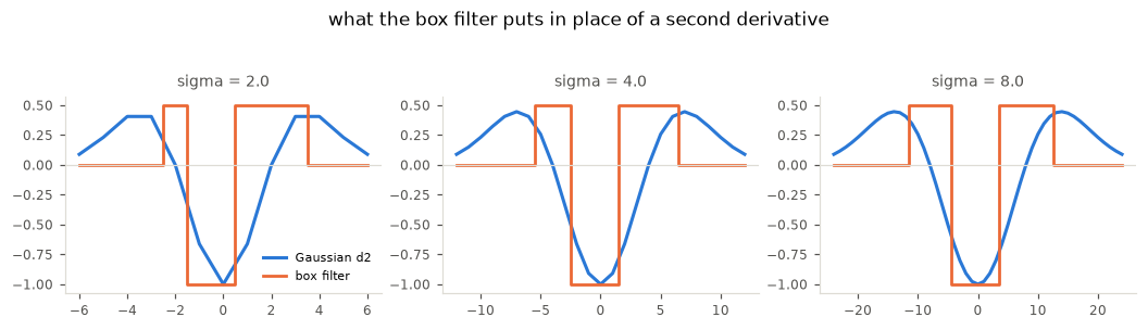

The box filter has the right gross shape — negative centre, positive flanks — and the wrong everything else: hard edges, no tails, and a width fixed by integer arithmetic rather than by sigma.

It is also not centred, for two separate reasons.

The first is integer geometry. mid starts at c - s2 with s2 = (size - 1) // 2 and runs size columns; side starts at c - s3 // 2 and runs s3. Where size is even, neither box can straddle the centre pixel, so the filter sits half a pixel off. The panels above show it: at sigma = 2 the negative lobe spans roughly -1.5 to +0.5 rather than -1 to +1. The source even has if size % 2 == 0: size += 1, but that line runs after s2, s3 and w are computed, so it has no effect on the filter.

The second is an off-by-one between _integ and integral_image. Skimage’s integral image has the same shape as the input, with S[m, n] = sum of X[i, j] for i <= m, j <= n. The four-corner formula in _integ is the OpenCV convention for a table of shape (H + 1, W + 1) with a leading row and column of zeros. On a same-shape table that formula sums the rectangle one pixel down and right of the corner it names. Every box in the filter therefore sits one pixel toward the bottom-right of (r, c), and a symmetric blob peaks when (r, c) is one pixel up and left of the true centre.

The half-pixel even-size term is real, but it is not what produces the constant (-1, -1) on discs: that offset appears at odd size too. Correcting the integral indexing shifts every box back by one pixel, and that is necessary. It is not sufficient, and the reason is the same parity argument applied to the other box.

mid runs size columns from c - s2 with s2 = (size - 1) // 2, so it straddles the centre pixel only when size is odd. side runs s3 columns from c - s3 // 2, so it straddles the centre only when s3 is odd. Both have to hold. The test is whether the response is symmetric about a symmetric blob’s true centre — the peak position of a flat response is arbitrary, its symmetry is not.

def det_variants(image, sigma, shifted):
    """`_hessian_matrix_det`, vectorised, with the `_integ` shift switchable."""
    size = int(3 * sigma)
    s2, s3, w = (size - 1) // 2, size // 3, size
    w_i = 1.0 / size / size
    n_rows, n_cols = image.shape
    table = np.zeros((n_rows + 1, n_cols + 1))
    table[1:, 1:] = image.cumsum(0).cumsum(1)
    off = 1 if shifted else 0            # `_integ` sums one pixel down and right

    def box(r, c, rl, cl):
        r0, c0 = np.clip(r + off, 0, n_rows), np.clip(c + off, 0, n_cols)
        r1, c1 = np.clip(r + off + rl, 0, n_rows), np.clip(c + off + cl, 0, n_cols)
        return np.maximum(0.0, table[r1, c1] + table[r0, c0]
                          - table[r0, c1] - table[r1, c0])

    rr, cc = np.indices(image.shape)
    dxy = -(box(rr - s3, cc + 1, s3, s3) + box(rr + 1, cc - s3, s3, s3)
            - box(rr - s3, cc - s3, s3, s3) - box(rr + 1, cc + 1, s3, s3)) * w_i
    dxx = -(box(rr - s3 + 1, cc - s2, 2 * s3 - 1, w)
            - 3 * box(rr - s3 + 1, cc - s3 // 2, 2 * s3 - 1, s3)) * w_i
    dyy = -(box(rr - s2, cc - s3 + 1, w, 2 * s3 - 1)
            - 3 * box(rr - s3 // 2, cc - s3 + 1, s3, 2 * s3 - 1)) * w_i
    return dxx * dyy - 0.81 * (dxy * dxy)

# The reimplementation is exact against the shipped routine in the interior,
# which is what licenses using it to reason about the shipped one.
probe_img = ski.util.img_as_float(ski.data.camera())[::4, ::4]
inner = (slice(30, -30),) * 2
worst = max(
    np.abs(hessian_matrix_det(probe_img, sigma=s, approximate=True)[inner]
           - det_variants(probe_img, s, shifted=True)[inner]).max()
    for s in (2.0, 3.0, 4.0)
)
print(f"vectorised reimplementation vs shipped, interior: max |difference| {worst:.1e}")

vectorised reimplementation vs shipped, interior: max |difference| 0.0e+00

SYM_N = 121
sym_centre = SYM_N // 2
sy, sx = np.indices((SYM_N, SYM_N))
sym_blob = np.exp(-((sy - sym_centre) ** 2 + (sx - sym_centre) ** 2) / (2 * 6.0**2))
SYM_PAD = 90
sym_padded = np.pad(sym_blob, SYM_PAD)


def asymmetry(sigma, shifted):
    """Departure from symmetry about the blob's true centre, padded so no clamping."""
    resp = det_variants(sym_padded, sigma, shifted)[SYM_PAD:-SYM_PAD, SYM_PAD:-SYM_PAD]
    return np.abs(resp - resp[::-1, ::-1]).max() / max(np.abs(resp).max(), 1e-30)


print(f"{'size':>5}{'s3':>5}{'size odd':>10}{'s3 odd':>8}"
      f"{'as shipped':>13}{'indexing fixed':>16}")
for size in range(3, 25):
    sigma = size / 3.0                      # so that int(3 * sigma) == size
    s3 = size // 3
    print(f"{size:>5}{s3:>5}{('yes' if size % 2 else 'no'):>10}"
          f"{('yes' if s3 % 2 else 'no'):>8}"
          f"{asymmetry(sigma, True):>12.1%}{asymmetry(sigma, False):>16.1%}")

 size   s3  size odd  s3 odd   as shipped  indexing fixed
    3    1       yes     yes       82.3%            0.0%
    4    1        no     yes       70.1%           40.3%
    5    1       yes     yes       37.6%            0.0%
    6    2        no      no      101.3%           81.3%
    7    2       yes      no       91.3%           74.3%
    8    2        no      no       89.4%           71.9%

    9    3       yes     yes       58.0%            0.0%

   10    3        no     yes      113.1%          115.7%
   11    3       yes     yes       38.8%            0.0%
   12    4        no      no       50.3%           84.1%
   13    4       yes      no       54.8%           77.2%
   14    4        no      no      108.6%          114.4%
   15    5       yes     yes       53.9%            0.0%

   16    5        no     yes       38.5%           25.5%

   17    5       yes     yes       66.8%            0.0%
   18    6        no      no       20.3%           44.8%
   19    6       yes      no       23.1%           35.1%
   20    6        no      no       27.4%           47.0%
   21    7       yes     yes       50.8%            0.0%
   22    7        no     yes       45.6%            8.5%
   23    7       yes     yes       53.4%            0.0%

   24    8        no      no       22.8%           28.5%

Fixing the indexing gives an exactly symmetric operator at every size where both size and s3 are odd, and leaves 35% to 77% asymmetry at size 7, 13 and 19 — the odd sizes whose s3 is even. So the centring defect is two separate parity conditions on top of the indexing shift, and a fix that addresses only the indexing still mis-centres a third of the odd scales.

Constraints on `size`¶

The filter is built from two widths that share one integer size:

size = int(3 * sigma)     # mid box width (also the filter's nominal width)
s3   = size // 3          # side / lobe width
s2   = (size - 1) // 2    # mid starts at c - s2

On the line of columns through the centre pixel c, each box is a half-open interval of pixels. Centred means the interval contains c and the same number of pixels on each side of c.

mid  :  [c - s2,  c - s2 + size)     width = size
side :  [c - s3 // 2,  c - s3 // 2 + s3)     width = s3

A half-open interval of odd length always has a unique middle pixel; one of even length never does. That is the whole constraint, applied twice.

def draw_box_row(ax, start, width, centre, label, colour, y=0.0):
    """One horizontal box on a 1-D pixel strip; shade pixels it covers."""
    xs = np.arange(centre - 8, centre + 9)
    for x in xs:
        face = colour if start <= x < start + width else "#f0eee8"
        ax.add_patch(plt.Rectangle((x - 0.5, y - 0.35), 1.0, 0.7,
                                   facecolor=face, edgecolor=GRID, lw=0.6))
    ax.axvline(centre, color=INK, lw=1.0, ls=":", zorder=3)
    ax.text(centre - 8.6, y, label, ha="right", va="center", fontsize=8,
            color=MUTED)
    covered = [x for x in xs if start <= x < start + width]
    left = covered[0] - centre if covered else None
    right = covered[-1] - centre if covered else None
    note = (f"[{start - centre:+d}, {start + width - centre:+d})"
            f"  →  {left:+d} … {right:+d}" if covered else "empty")
    ax.text(centre + 8.6, y, note, ha="left", va="center", fontsize=7,
            color=MUTED, family="monospace")


def panel_boxes(ax, size, title):
    s2, s3 = (size - 1) // 2, size // 3
    c = 0
    draw_box_row(ax, c - s2, size, c, f"mid  size={size}", C_ONE, y=0.8)
    draw_box_row(ax, c - s3 // 2, s3, c, f"side s3={s3}", C_TWO, y=0.0)
    mid_ok = size % 2 == 1
    side_ok = s3 % 2 == 1
    ax.set_xlim(-9.5, 12.5)
    ax.set_ylim(-0.7, 1.4)
    ax.set_aspect("equal")
    bare(ax, title)
    verdict = ("both centred" if mid_ok and side_ok
               else "mid off" if not mid_ok and side_ok
               else "side off" if mid_ok and not side_ok
               else "both off")
    ax.text(0, -0.55, verdict, ha="center", va="top", fontsize=8,
            color=C_THREE if mid_ok and side_ok else C_TWO)


fig, axes = plt.subplots(2, 2, figsize=(9.2, 3.6))
for ax, size, title in zip(
        axes.ravel(),
        (8, 9, 7, 5),
        ("even size: mid cannot straddle c",
         "size=9, s3=3: both odd → centred",
         "size=7 ≡ 1 (mod 6): s3 even → side off",
         "size=5 ≡ 5 (mod 6): both odd → centred")):
    panel_boxes(ax, size, title)
fig.suptitle("which pixels mid and side cover, relative to the centre c", y=1.02)
fig.tight_layout()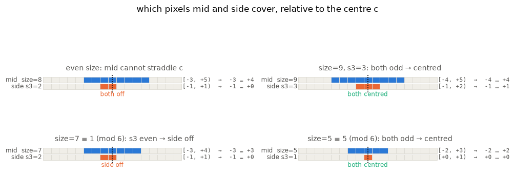

Read each strip from the colon at c. An odd-width box paints the same count of cells left and right of that line; an even-width box always has one extra cell on one side. For size = 8 the mid box is the even case. For size = 7, mid is fine (7 is odd) but s3 = 2 is even, so the side lobe sits half a pixel off — that is the residual asymmetry after D1.

Every odd integer is congruent to 1, 3 or 5 modulo 6. Only those three classes need checking, because even size already fails the mid condition.

# size = 6k+r. For odd size, r ∈ {1, 3, 5}.
print(f"{'size':>5}{'mod 6':>7}{'s3':>5}{'s3 =':>14}{'s3 odd?':>9}{'centred?':>10}")
for size in range(3, 25):
    if size % 2 == 0:
        continue
    r = size % 6
    s3 = size // 3
    # Algebra: (6k+1)//3 = 2k even; (6k+3)//3 = 2k+1 odd; (6k+5)//3 = 2k+1 odd.
    form = {1: "2k (even)", 3: "2k+1 (odd)", 5: "2k+1 (odd)"}[r]
    ok = s3 % 2 == 1
    print(f"{size:>5}{r:>7}{s3:>5}{form:>14}{('yes' if ok else 'no'):>9}"
          f"{('yes' if ok else 'NO'):>10}")

 size  mod 6   s3          s3 =  s3 odd?  centred?
    3      3    1    2k+1 (odd)      yes       yes
    5      5    1    2k+1 (odd)      yes       yes
    7      1    2     2k (even)       no        NO
    9      3    3    2k+1 (odd)      yes       yes
   11      5    3    2k+1 (odd)      yes       yes
   13      1    4     2k (even)       no        NO
   15      3    5    2k+1 (odd)      yes       yes
   17      5    5    2k+1 (odd)      yes       yes
   19      1    6     2k (even)       no        NO
   21      3    7    2k+1 (odd)      yes       yes
   23      5    7    2k+1 (odd)      yes       yes

So:

residue of `size` mod 6	examples	`size` odd?	`s3` odd?	usable?
`0, 2, 4`	6, 8, 10	no	—	no (mid off)
`1`	7, 13, 19	yes	no	no (side off)
`3`	3, 9, 15, 21	yes	yes	yes
`5`	5, 11, 17, 23	yes	yes	yes

“Not 1 mod 6” is the short name for the last two rows together: odd sizes whose remainder on division by 6 is 3 or 5. SURF’s own ladder 9, 15, 21, 27, … is the stricter subset with residue 3 only (and step 6).

fig, ax = plt.subplots(figsize=(9.0, 1.8))
for size in range(3, 28):
    r = size % 6
    if size % 2 == 0:
        colour, tag = GRID, "even"
    elif r == 1:
        colour, tag = C_TWO, "1 mod 6"
    else:
        colour, tag = C_THREE, "valid"
    ax.add_patch(plt.Rectangle((size - 0.4, 0), 0.8, 1.0,
                               facecolor=colour, edgecolor="white", lw=0.5))
    ax.text(size, 0.5, str(size), ha="center", va="center", fontsize=7,
            color="white" if colour != GRID else MUTED)
ax.set_xlim(2.3, 27.7)
ax.set_ylim(-0.2, 1.6)
ax.set_yticks([])
ax.set_xticks([])
for spine in ax.spines.values():
    spine.set_visible(False)
ax.plot([], [], color=C_THREE, lw=6, label="valid (3 or 5 mod 6)")
ax.plot([], [], color=C_TWO, lw=6, label="odd but 1 mod 6 — side off")
ax.plot([], [], color=GRID, lw=6, label="even — mid off")
ax.legend(frameon=False, fontsize=7, loc="upper center",
          bbox_to_anchor=(0.5, 1.35), ncol=3)
ax.set_xlabel("size = int(3 · sigma)", fontsize=8, color=MUTED)
fig.tight_layout()

The dead size += 1 line only moves even sizes into the odd column. It turns 8 → 9 (good) but also leaves 7 untouched, and would turn 6 → 7 (still bad). A D2 fix has to land in the green set above, not merely in the odd integers.

DETECTORS = {"blob_dog": lambda im: blob_dog(im, min_sigma=2, max_sigma=30,
                                             threshold=0.05),
             "blob_log": lambda im: blob_log(im, min_sigma=2, max_sigma=30,
                                             num_sigma=30, threshold=0.05),
             "blob_doh": lambda im: blob_doh(im, min_sigma=2, max_sigma=30,
                                             num_sigma=30, threshold=0.005)}

print("offset of the reported centre from the true centre, in pixels")
print(f"{'true radius':>12}" + "".join(f"{n:>20}" for n in DETECTORS))
for r0, c0, radius in TRUTH:
    line = f"{radius:>12}"
    for name, run in DETECTORS.items():
        near = [b for b in run(discs)
                if (b[0] - r0) ** 2 + (b[1] - c0) ** 2 < 400]
        if not near:
            line += f"{'missed':>20}"
            continue
        b = min(near, key=lambda b: (b[0] - r0) ** 2 + (b[1] - c0) ** 2)
        line += f"{f'{b[0] - r0:+.0f}, {b[1] - c0:+.0f}':>20}"
    print(line)

offset of the reported centre from the true centre, in pixels
 true radius            blob_dog            blob_log            blob_doh

           6              +0, +0              +0, +0              -1, -1

          10              +0, +0              +0, +0              -1, -1

          16              +0, +0              +0, +0              -1, -1

          24              +0, +0              +0, +0              -1, -1

blob_dog and blob_log land on the centre exactly. blob_doh is one pixel up and one pixel left, at every radius — including radii whose int(3 * sigma) is odd. Over random centres and radii the column offset is -1 every time and the row offset is -1 almost every time.

rng = np.random.default_rng(0)
small_n = 300
sr, sc = np.indices((small_n, small_n))
offsets = []
for _ in range(12):
    r0, c0 = int(rng.integers(60, 240)), int(rng.integers(60, 240))
    radius = int(rng.integers(5, 20))
    one = np.zeros((small_n, small_n))
    one[(sr - r0) ** 2 + (sc - c0) ** 2 <= radius**2] = 1.0
    near = [b for b in blob_doh(one, min_sigma=2, max_sigma=30, num_sigma=30,
                                threshold=0.005)
            if (b[0] - r0) ** 2 + (b[1] - c0) ** 2 < 900]
    if near:
        b = min(near, key=lambda b: (b[0] - r0) ** 2 + (b[1] - c0) ** 2)
        offsets.append((b[0] - r0, b[1] - c0))

offsets = np.array(offsets)
print(f"{len(offsets)} blobs over random centres and radii")
seen = sorted({(float(a), float(b)) for a, b in offsets})
print("   distinct offsets : "
      + ", ".join(f"({a:+.0f}, {b:+.0f})" for a, b in seen))
print(f"   mean offset      : {offsets.mean(axis=0)}")

12 blobs over random centres and radii
   distinct offsets : (-1, -1), (+0, -1)
   mean offset      : [-0.91666667 -1.        ]

A constant offset is the easiest kind of defect to fix and the easiest to miss, because every blob moves together and the picture still looks right.

# `_integ`'s four-corner formula on a same-shape integral, vs the sum it names.
probe = np.arange(1.0, 26.0).reshape(5, 5)
ii = ski.transform.integral_image(probe)
r, c, rl, cl = 1, 1, 2, 2
named = probe[r:r + rl, c:c + cl].sum()
formula = ii[r, c] + ii[r + rl, c + cl] - ii[r, c + cl] - ii[r + rl, c]
shifted = probe[r + 1:r + rl + 1, c + 1:c + cl + 1].sum()
print(f"sum of the named window     : {named:.0f}")
print(f"four-corner formula on ii   : {formula:.0f}")
print(f"sum one pixel down and right: {shifted:.0f}")

sum of the named window     : 40
four-corner formula on ii   : 64
sum one pixel down and right: 64

6. The scale axis is quantised¶

size = int(3 * sigma) is the whole dependence on sigma, and it is an integer. Distinct scales therefore collapse onto the same filter.

photo = ski.util.img_as_float(ski.data.camera())[::2, ::2]
base = hessian_matrix_det(photo, sigma=3.0, approximate=True)

print(f"{'sigma':>8}{'int(3*sigma)':>14}{'identical to sigma = 3.0':>28}")
for sigma in (3.0, 3.2, 3.32, 3.34, 3.67, 4.0):
    got = hessian_matrix_det(photo, sigma=sigma, approximate=True)
    print(f"{sigma:>8}{int(3 * sigma):>14}{str(np.array_equal(got, base)):>28}")

   sigma  int(3*sigma)    identical to sigma = 3.0
     3.0             9                        True
     3.2             9                        True
    3.32             9                        True
    3.34            10                       False
    3.67            11                       False
     4.0            12                       False

Asking for sigma = 3.0, 3.2 or 3.32 returns bit-identical planes. The scale axis moves in steps of one third, so a num_sigma finer than that buys duplicate work and nothing else — and the duplicates still count towards the maximum search.

Below sigma = 1 the lobe collapses to zero and the response vanishes altogether.

small = np.exp(-((rows[:81, :81] - 40) ** 2 + (cols[:81, :81] - 40) ** 2) / 32)
print(f"{'sigma':>7}{'size':>6}{'lobe':>6}{'centre response':>18}")
for sigma in (0.5, 0.9, 1.0, 2.0, 4.0):
    size = int(3 * sigma)
    got = hessian_matrix_det(small, sigma=sigma, approximate=True)[40, 40]
    print(f"{sigma:>7}{size:>6}{size // 3:>6}{got:>18.3e}")

  sigma  size  lobe   centre response
    0.5     1     0         0.000e+00
    0.9     2     0         0.000e+00
    1.0     3     1         3.442e-05
    2.0     6     2         3.294e-03
    4.0    12     4         1.634e-02

The docstring warns that the method “can’t be used for detecting blobs of radius less than 3px”, which is this. It is documented, and it is a hard floor rather than a gradual loss.

7. Scale selection, measured¶

The test that matters is whether the response peaks at the right scale. For comparison, here is the same determinant computed exactly, with the corrected Gaussian kernels of on_hessian.md.

def gaussian_taps(sigma, order, trunc=8):
    lw = int(trunc * sigma + 0.5)
    x = np.arange(-lw, lw + 1).astype(float)
    g = np.exp(-(x**2) / (2 * sigma**2))
    g /= g.sum()
    if order == 0:
        return x, g
    if order == 1:
        return x, g * (x / sigma**2)
    return x, g * ((x**2 - sigma**2) / sigma**4)


def corrected_taps(sigma, order, trunc=8):
    """Fix C of `on_hessian.md`: repair the discrete moments."""
    x, g = gaussian_taps(sigma, 0, trunc)
    _, k = gaussian_taps(sigma, order, trunc)
    if order == 0:
        return x, g
    if order == 1:
        return x, k / (k * x).sum()
    k = k - k.sum() * g
    return x, k / ((k * x**2).sum() / 2)


def exact_doh(image, sigma, mode="nearest", trunc=8):
    """Scale-normalised determinant of the Hessian, exact kernels."""
    taps = {o: corrected_taps(sigma, o, trunc)[1] for o in (0, 1, 2)}
    sep = lambda a, b: ndi.correlate1d(
        ndi.correlate1d(image, taps[a], axis=0, mode=mode), taps[b], axis=1, mode=mode)
    hrr, hrc, hcc = sep(2, 0), sep(1, 1), sep(0, 2)
    return (sigma**4) * (hrr * hcc - hrc**2)


def box_doh(image, sigma):
    """The box-filter determinant, by the public route.

    `hessian_matrix_det(..., approximate=True)` builds the integral image and
    calls the same routine `blob_doh` uses; the two agree bit for bit.
    """
    return hessian_matrix_det(image, sigma=sigma, approximate=True)


def best_of(f, n=5):
    """Minimum of `n` timed calls, after one warmup call."""
    f()
    times = []
    for _ in range(n):
        t0 = time.perf_counter()
        f()
        times.append(time.perf_counter() - t0)
    return min(times)

M = 201
mc = M // 2
mr2 = (np.indices((M, M))[0] - mc) ** 2 + (np.indices((M, M))[1] - mc) ** 2
trial = np.geomspace(1.0, 14.0, 50)


def gaussian_blob(width):
    return np.exp(-mr2 / (2 * width**2)) / (2 * np.pi * width**2)


print(f"{'blob width':>12}{'ideal':>8}{'box filters':>14}{'exact':>9}")
for width in (1.5, 2.0, 3.0, 5.0, 8.0):
    target = gaussian_blob(width)
    picks = [trial[int(np.argmax([f(target, s)[mc, mc] for s in trial]))]
             for f in (box_doh, exact_doh)]
    print(f"{width:>12}{width:>8.2f}{picks[0]:>14.2f}{picks[1]:>9.2f}")

  blob width   ideal   box filters    exact

         1.5    1.50          2.01     1.54

         2.0    2.00          4.06     2.01

         3.0    3.00          6.24     2.94

         5.0    5.00          8.17     5.03

         8.0    8.00         14.00     8.17

fig, axes = plt.subplots(1, 2, figsize=(8.0, 3.2), sharey=True)
for ax, (name, f) in zip(axes, (("box filters", box_doh), ("exact", exact_doh))):
    for width, colour in ((1.5, C_ONE), (3.0, C_TWO), (8.0, C_THREE)):
        target = gaussian_blob(width)
        resp = np.array([f(target, s)[mc, mc] for s in trial])
        resp = resp / np.abs(resp).max()
        ax.plot(trial, resp, color=colour, lw=1.9, label=f"width {width}")
        ax.axvline(width, color=colour, lw=0.9, ls=":")
        ax.plot([trial[int(np.argmax(resp))]], [resp.max()], "o", color=colour,
                markersize=6, markeredgecolor="white", zorder=5)
    ax.set_xscale("log")
    ax.set_xlabel("sigma", fontsize=8, color=MUTED)
    recede(ax, name)
axes[0].set_ylabel("normalised response", fontsize=8, color=MUTED)
axes[0].legend(frameon=False, fontsize=7, loc="upper left")
fig.suptitle("dotted line: the blob's true width.   circle: where the method "
             "puts it", y=1.04)
fig.tight_layout()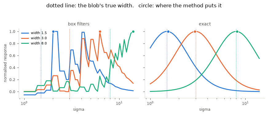

The exact determinant lands on each dotted line. The box version reads high and increasingly so, running into the top of the axis for the widest blob. That is the +5% to +33% of section 3, seen at its source.

8. The border¶

print(f"{'sigma':>6}{'box filters':>14}{'exact':>10}")
for sigma in (2.0, 4.0, 8.0):
    pad = 2 * int(8 * sigma + 0.5) + 1
    big = np.pad(photo, pad, mode="edge")
    row = ""
    for f in (box_doh, exact_doh):
        reference = f(big, sigma)[pad:-pad, pad:-pad]
        gap = np.abs(f(photo, sigma) - reference)
        row += f"{gap.max() / max(np.abs(reference).max(), 1e-12):>13.1%}"
    print(f"{sigma:>6}{row}")

 sigma   box filters     exact
   2.0        83.1%         0.0%
   4.0        45.2%         0.0%
   8.0        86.9%         0.0%

The exact route is exact at the border, for the reason on_hessian.md section 7 sets out: one filter call per element, so the boundary rule is applied once. The box route is not. The rest of this section diagnoses why, and what a fix costs.

What `_integ` does at the edge¶

Every box sum goes through _integ, which clips each corner of the requested rectangle to the image and then applies the four-corner integral formula. There is no mode, and no pad. A rectangle that sticks out is never extended — but what happens to it instead depends on which edge it crosses, and the two outcomes are different failures.

_integ clips the origin first and only then adds the extent:

r  = clip(r,      0, rows - 1)
r2 = clip(r + rl, 0, rows - 1)

Because r + rl is measured from the already clipped r, a box hanging off the top or left keeps its full size and is slid inward. A box hanging off the bottom or right has nowhere to slide, so r2 clips and it is shrunk.

Both are wrong, and they are wrong in different ways. The slid box computes a correctly normalised derivative of the wrong neighbourhood, displaced toward the interior. The shrunk box computes over fewer taps than the (1, -2, 1) balance assumes, while still dividing by size ** 2 as though the full box were present — so its normalisation no longer matches the area actually summed.

def pad_needed(sigma):
    """Half-width the filter can reach past a pixel, in pixels.

    From the rectangle list in `_hessian_matrix_det`: the farthest look is
    `size - (size - 1) // 2` (the `dyy` mid box runs `size` rows from
    `r - s2`).
    """
    size = int(3 * sigma)
    return size - (size - 1) // 2


def clamped_box(r, c, rl, cl, shape):
    """Origin and extent `_integ` actually integrates over, given a request."""
    rows, cols = shape

    def clip(x, lo, hi):
        return hi if x > hi else (lo if x < lo else x)

    r0, c0 = clip(r, 0, rows - 1), clip(c, 0, cols - 1)
    # `_integ` measures the extent from the clipped origin, not the requested one.
    r1, c1 = clip(r0 + rl, 0, rows - 1), clip(c0 + cl, 0, cols - 1)
    return (r0, c0), (r1 - r0, c1 - c0)


def draw_integ_edge(ax, shape, request, title):
    """Requested rectangle vs what `_integ` actually sums after clip-then-extent."""
    rows, cols = shape
    r, c, rl, cl = request
    (r0, c0), (h, w) = clamped_box(r, c, rl, cl, shape)

    # Image pixels.
    for i in range(rows):
        for j in range(cols):
            ax.add_patch(plt.Rectangle(
                (j - 0.5, i - 0.5), 1, 1,
                facecolor="#f0eee8", edgecolor=GRID, lw=0.7))

    # Requested box (may leave the image).
    ax.add_patch(plt.Rectangle(
        (c - 0.5, r - 0.5), cl, rl,
        fill=False, edgecolor=C_TWO, lw=2.0, ls="--", zorder=3,
        label="requested"))
    # Actual summed region.
    if h > 0 and w > 0:
        ax.add_patch(plt.Rectangle(
            (c0 - 0.5, r0 - 0.5), w, h,
            facecolor=C_ONE, alpha=0.45, edgecolor=C_ONE, lw=1.8, zorder=2,
            label="actually summed"))

    ax.set_xlim(-2.5, cols + 1.5)
    ax.set_ylim(rows + 1.5, -2.5)          # array order: row 0 at the top
    ax.set_aspect("equal")
    ax.set_xticks(range(cols))
    ax.set_yticks(range(rows))
    ax.tick_params(labelsize=7, colors=MUTED)
    for spine in ax.spines.values():
        spine.set_color(GRID)
    ax.set_title(title, fontsize=8)

    # Annotate the clip arithmetic on the vertical axis of this request.
    ax.annotate(
        f"ask [{r}, {r + rl}) → integ [{r0}, {r0 + h})",
        xy=(cols / 2 - 0.5, -1.6), ha="center", va="top",
        fontsize=7, color=MUTED, family="monospace")


# Toy geometry: a 5×4 box on an 8×8 image, overhanging by two pixels.
SHAPE = (8, 8)
BOX = (5, 4)                               # (rl, cl)
fig, axes = plt.subplots(1, 2, figsize=(8.4, 4.0))
draw_integ_edge(
    axes[0], SHAPE, (-2, 2, *BOX),
    "top: origin clips, extent kept → slid inward")
draw_integ_edge(
    axes[1], SHAPE, (5, 2, *BOX),
    "bottom: origin stays, extent clips → shrunk")
handles, labels = axes[0].get_legend_handles_labels()
fig.legend(handles, labels, frameon=False, fontsize=8,
           loc="upper center", ncol=2, bbox_to_anchor=(0.5, 1.02))
fig.suptitle("`_integ` on the same 5×4 request, opposite edges", y=1.08)
fig.tight_layout()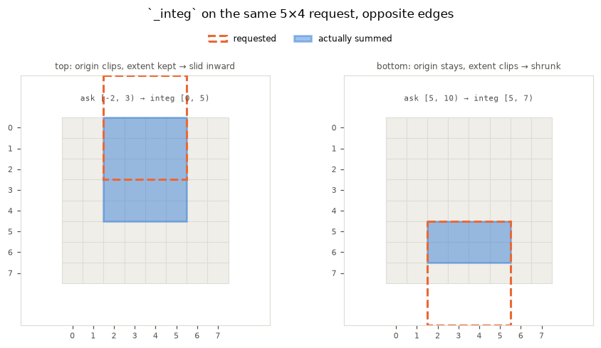

The dashed outline is what the filter asked for; the filled region is what the four-corner sum actually covers. On the top, clipping the origin to 0 and then adding rl slides a full-size box into the image. On the bottom, the origin is already legal, so r + rl hits the far bound and the height collapses. Left and right edges behave the same way as top and bottom, on columns.

sigma = 4.0
size = int(3 * sigma)
s2, s3 = (size - 1) // 2, size // 3
asked = (size, 2 * s3 - 1)
print(f"sigma = {sigma}, size = {size}, pad_needed = {pad_needed(sigma)}")
print(f"the dyy mid box asks for {asked[0]} x {asked[1]}\n")

rows, cols = photo.shape
for label, (r, c) in (("top-left     (0, 0)", (0, 0)),
                      (f"bottom-right ({rows - 1}, {cols - 1})", (rows - 1, cols - 1))):
    origin, extent = clamped_box(r - s2, c - s3 + 1, size, 2 * s3 - 1, photo.shape)
    verdict = "slid, full size" if extent == asked else "shrunk"
    print(f"   {label}: origin {origin}, extent {extent}  -> {verdict}")

sigma = 4.0, size = 12, pad_needed = 7
the dyy mid box asks for 12 x 7

   top-left     (0, 0): origin (0, 0), extent (12, 7)  -> slid, full size
   bottom-right (255, 255): origin (250, 252), extent (5, 3)  -> shrunk

The same box, the same distance outside the image, and two different outcomes. Only the bottom-right one loses taps; the top-left one keeps all of them and looks somewhere else instead. Neither is the filter the caller asked for, and neither is what any mode would give.

The defect is a band, not a haze¶

sigma = 4.0
need = pad_needed(sigma)
pad = 2 * int(8 * sigma + 0.5) + 1
reference = box_doh(np.pad(photo, pad, mode="edge"), sigma)[pad:-pad, pad:-pad]
gap = np.abs(box_doh(photo, sigma) - reference)

rr, cc = np.indices(photo.shape)
dist = np.minimum(np.minimum(rr, cc),
                  np.minimum(photo.shape[0] - 1 - rr, photo.shape[1] - 1 - cc))

print(f"{'dist to border':>16}{'max |error|':>14}")
for d in range(need + 2):
    band = gap[dist == d]
    print(f"{d:>16}{band.max():>14.3e}")

  dist to border   max |error|
               0     1.196e-02
               1     1.028e-02
               2     1.097e-02
               3     1.005e-02
               4     7.630e-03
               5     4.972e-03
               6     2.532e-03
               7     3.788e-14
               8     3.263e-14

fig, axes = plt.subplots(1, 3, figsize=(9.6, 3.2))
bare(axes[0], "response, as shipped")
axes[0].imshow(box_doh(photo, sigma), cmap=SEQ)
bare(axes[1], "pad-once reference")
axes[1].imshow(reference, cmap=SEQ)
bare(axes[2], "|shipped − reference|")
axes[2].imshow(gap, cmap=SEQ)
fig.suptitle(f"sigma = {sigma}: error lives in a {need}-pixel border band", y=1.04)
fig.tight_layout()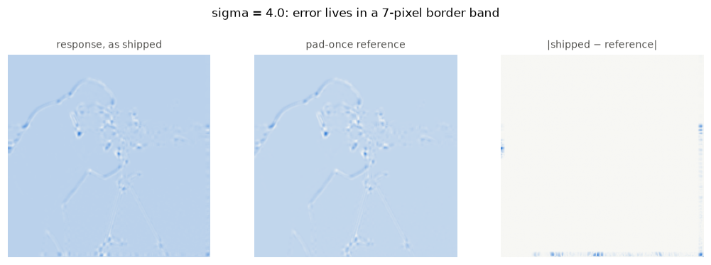

Inside dist >= pad_needed(sigma) the two agree to numerical noise. Outside, the relative error reaches tens of percent of the peak response. On a 256×256 image that band is about 6% of the pixels at sigma = 2 and about 35% at sigma = 16.

This is a different border defect from the one in hessian_matrix (on_hessian.md). There, a boundary rule is applied, but twice, so the second pass invents values. Here no boundary rule is applied at all: the filter itself changes shape.

Fix: pad once, then crop¶

Extend the image by pad_needed(sigma) under the chosen boundary rule, build the integral image on that padded array, run the existing box filters, and crop back. Every surviving pixel then sees a full-size filter over edge-extended data — the same construction the measurement above uses as its reference.

def box_doh_padded(image, sigma, mode="edge"):
    """Approximate DoH with a single boundary extension."""
    p = pad_needed(sigma)
    return box_doh(np.pad(image, p, mode=mode), sigma)[p:-p, p:-p]


print(f"{'sigma':>6}{'as shipped':>14}{'pad once':>12}{'pad':>6}")
for sigma in (2.0, 4.0, 8.0, 16.0):
    p_ref = 2 * int(8 * sigma + 0.5) + 1
    reference = box_doh(np.pad(photo, p_ref, mode="edge"),
                        sigma)[p_ref:-p_ref, p_ref:-p_ref]
    scale = max(np.abs(reference).max(), 1e-12)
    shipped = np.abs(box_doh(photo, sigma) - reference).max() / scale
    fixed = np.abs(box_doh_padded(photo, sigma) - reference).max() / scale
    print(f"{sigma:>6}{shipped:>13.1%}{fixed:>12.1e}{pad_needed(sigma):>6}")

 sigma    as shipped    pad once   pad
   2.0        83.1%     9.1e-12     4
   4.0        45.2%     2.0e-12     7
   8.0        86.9%     2.5e-12    13

  16.0       101.2%     1.4e-12    25

print(f"{'sigma':>6}{'pad':>6}{'as shipped':>12}{'pad once':>10}{'cost':>8}")
for sigma in (2.0, 4.0, 8.0, 16.0):
    p = pad_needed(sigma)
    t_now = best_of(lambda: box_doh(photo, sigma))
    t_pad = best_of(lambda: box_doh_padded(photo, sigma))
    print(f"{sigma:>6}{p:>6}{t_now * 1e3:>9.2f} ms{t_pad * 1e3:>7.2f} ms"
          f"{t_pad / t_now:>7.2f}x")

 sigma   pad  as shipped  pad once    cost
   2.0     4     1.45 ms   1.25 ms   0.86x
   4.0     7     1.45 ms   1.30 ms   0.90x
   8.0    13     1.45 ms   1.42 ms   0.98x
  16.0    25     1.45 ms   1.65 ms   1.14x

The cost is a few tens of percent on this 256×256 photograph, not an order of magnitude. The box-filter property — cost independent of sigma in the filter itself — is preserved; only the padded area grows with sigma, and linearly.

Two alternatives are worse for this function:

Replace the boxes with exact Gaussian derivatives. That clears the border, and the scale bias, and the position offset, but it destroys the flat-cost reason blob_doh exists. blob_log already is that detector.
Only set exclude_border in the peak search. That hides false maxima in the bad band; it does not make the response correct for any pixel that still uses a shrunk filter, and it throws away a growing fraction of the image as sigma grows.

The pad-once fix is local to hessian_matrix_det(..., approximate=True) (or to the wrapper that builds its integral image). It does not repair the one-pixel position offset in the interior: that is the _integ indexing defect of section 5, and it needs its own change.

9. What the approximation buys¶

print(f"{'sigma':>6}{'box filters':>14}{'exact':>11}{'ratio':>9}")
for sigma in (2.0, 4.0, 8.0, 16.0):
    t_box = best_of(lambda: box_doh(photo, sigma))
    t_exact = best_of(lambda: exact_doh(photo, sigma))
    print(f"{sigma:>6}{t_box * 1e3:>11.2f} ms{t_exact * 1e3:>8.2f} ms"
          f"{t_exact / t_box:>8.1f}x")

 sigma   box filters      exact    ratio
   2.0       1.45 ms    5.53 ms     3.8x

   4.0       1.43 ms   10.09 ms     7.1x

   8.0       1.43 ms   16.83 ms    11.8x

  16.0       1.42 ms   29.98 ms    21.1x

This is the trade, and it is a real one. The box cost is flat: the same rectangle count whatever sigma is. The exact cost grows linearly with sigma, because the kernel does. At sigma = 16 the gap is already fortyfold and it keeps widening.

So replacing the box filters with exact kernels would fix the scale bias and the border, and destroy the reason blob_doh exists. blob_log is already the accurate Gaussian-based detector; a blob_doh that computed exact Gaussian derivatives would be a slower blob_log under a different name.

10. Do the `hessian_matrix` fixes reach it?¶

No. on_hessian.md finds a border defect in hessian_matrix that reaches frangi, sato, meijering and hessian, and proposes fixes A and C. None of them touches blob_doh, which calls _hessian_matrix_det directly.

hessian_matrix_det is the function to watch, because it has two paths.

print(f"{'sigma':>6}{'approximate=True':>20}{'approximate=False':>21}")
for sigma in (1.0, 2.0, 4.0):
    pad = 2 * int(8 * sigma + 0.5) + 1
    big = np.pad(photo, pad, mode="edge")
    row = ""
    for approximate in (True, False):
        direct = hessian_matrix_det(photo, sigma=sigma, approximate=approximate)
        reference = hessian_matrix_det(big, sigma=sigma,
                                       approximate=approximate)[pad:-pad, pad:-pad]
        gap = np.abs(direct - reference)
        row += f"{gap.max() / max(np.abs(reference).max(), 1e-12):>19.1%}"
    print(f"{sigma:>6}{row}")

 sigma    approximate=True    approximate=False

   1.0              93.6%              67.0%
   2.0              83.1%              64.1%
   4.0              45.2%              86.5%

approximate=False routes through hessian_matrix, so it inherits the border defect and fixes A and C repair it. approximate=True is the box route, with a larger border problem of its own that no fix in on_hessian.md addresses.

11. How other libraries do it¶

OpenCV has no direct equivalent of this trio. cv2.SimpleBlobDetector is not a scale-space method at all — it thresholds the image at a series of levels and groups the connected components, so it finds regions rather than scales.

params = cv2.SimpleBlobDetector_Params()
params.filterByArea, params.minArea, params.maxArea = True, 50, 5000
params.filterByCircularity = params.filterByConvexity = False
params.filterByInertia = params.filterByColor = False
detector = cv2.SimpleBlobDetector_create(params)

keypoints = detector.detect((discs * 255).astype(np.uint8))
print(f"{'true radius':>12}{'SimpleBlobDetector':>22}")
for r0, c0, radius in TRUTH:
    near = [k for k in keypoints
            if (k.pt[1] - r0) ** 2 + (k.pt[0] - c0) ** 2 < 400]
    got = near[0].size / 2 if near else np.nan
    print(f"{radius:>12}{got:>13.1f} ({(got - radius) / radius:+.0%})")

 true radius    SimpleBlobDetector
           6          5.5 (-8%)
          10          9.5 (-5%)
          16         15.5 (-3%)
          24         23.4 (-2%)

It recovers the radii of solid discs well, because a disc is exactly what it looks for. It has no scale-normalised response, so it cannot rank a blob’s strength across scale, and it does not generalise to blobs that are not threshold-separable from their surroundings.

cv2.SIFT uses a difference of Gaussians, like blob_dog, with the same sigma_ratio trade for the same reason. The genuine SURF implementation, which is what blob_doh reproduces, sits in opencv-contrib behind a build flag and is not available here.

12. What to do¶

blob_dog. Nothing. Its bias is the documented sigma_ratio approximation, it shrinks when the caller asks for it to, and it matches what SIFT does.

blob_log. Nothing. It is the accurate detector of the three.

blob_doh. Four defects, and they are genuinely independent: each has its own cause, its own patch, and its own blast radius. Fixing one does not disturb another, so they can go in separately and in any order.

#	defect	cause	fix	changes output
D1	every blob reported one pixel up and left	`_integ`’s four-corner formula assumes a zero-padded `(H+1, W+1)` table; skimage’s integral image is same-shape, so each box sums one pixel down and right of the corner it names	index the integral image correctly, or build a zero-padded one	positions move by one pixel, everywhere
D2	boxes still off-centre at some scales	`mid` needs `size` odd, `side` needs `s3 = size // 3` odd; the `size += 1` line meant to fix this is dead, and neither condition is enforced	choose `size` so both are odd	responses change at the affected scales
D3	reported radius `+5%` to `+33%`	`size = int(3 * sigma)` does not reproduce SURF’s own filter-size-to-scale relation	recalibrate the constant	reported radii shrink
D4	border band wrong by 45% to 101%	`_integ` clips instead of extending: boxes slide at the top and left, shrink at the bottom and right, with no `mode`	pad by `size - (size - 1) // 2` under the chosen rule, filter, crop	a border band changes; the interior does not

D1 first. It is the smallest patch and the clearest bug — an integral-image convention mismatch, not an approximation anyone chose. It is also a prerequisite for testing D2, because while every box is displaced by a pixel there is no clean centre to measure parity against.

D2 needs a decision, not just a patch. Both size and size // 3 must be odd — see Constraints on size above for the geometry and the residue table. The smallest fix is to round size up to the next value satisfying both — size ∈ {3, 5, 9, 11, 15, 17, 21, 23, …}, i.e. odd and not 1 mod 6. That coarsens the scale axis further, which interacts with D3: recalibrating the size-to-sigma constant and constraining the realisable sizes are the same conversation, and doing them in one change is cheaper than doing them twice.

D4 is self-contained and the measurements in section 8 are ready to become a test: exact agreement with a pad-once reference outside pad_needed(sigma), 1.15x to 1.38x cost on a 256x256 image, flat-cost property preserved.

The quantised scale axis is not on the list because it is not a defect to fix. num_sigma finer than one third silently computes duplicate planes; a docstring line, or rounding sigma_list onto the realisable grid, is the whole remedy. D2 makes the grid coarser still, so document it after D2 lands.

Would exact kernels be better, given `on_hessian` fixes A and C?¶

Worth asking, because that notebook’s fixes change the arithmetic on the other side of the comparison. Fix A computes each Hessian element in one gaussian_filter call; Fix C repairs the discrete moments of the second derivative kernel and, in doing so, removes the need for truncate = 100 at small sigma. Together they make the exact route both correct at the border and much faster than it was — the exact_doh used in sections 7 to 9 above is already built on them.

It still is not the answer for blob_doh, and the timing table in section 9 is why: even with A and C the exact route costs 4.6x at sigma = 2 and 41.6x at sigma = 16, because its kernels grow with sigma while the box filters do not. The gap widens without limit. A blob_doh built on exact kernels would fix D1 through D4 at a stroke and would be a slower blob_log wearing a different name.

Where A and C do land is hessian_matrix_det(..., approximate=False), which routes through hessian_matrix and inherits both. That path needs nothing from this notebook. The split to hold onto is: approximate=False is fixed by the on_hessian work, approximate=True and blob_doh need D1 to D4, and no fix crosses between them.

Measured with scikit-image from this working tree, OpenCV 5.0.0, on 400x400 synthetic discs and the 256x256 camera photograph.

References¶

Bay, H., Tuytelaars, T., & Van Gool, L. (2006). SURF: Speeded Up Robust Features. In Computer Vision – ECCV 2006 (pp. 404–417). Springer Berlin Heidelberg. 10.1007/11744023_32