Meijering neuriteness: paper fidelity and the scale normalisation

Meijering et al. (2004) define a single-scale neuriteness with one global normaliser. skimage.filters.meijering adds a multiscale loop and divides each scale by its own maximum. This notebook checks the single-scale fidelity, then measures what the multiscale normalisation does to detection and to width, and which normalisation a multiscale API should use.

Coordinates are array order. Bright ridges use black_ridges=False. The alpha sign is settled in meijering_alpha.md; this notebook uses the paper value alpha = -1/3 unless a cell says otherwise. The paper is Meijering et al., Cytometry A 58:167-176 (2004); the authors’ implementation is NeuronJ.

1. Setup¶

import numpy as np
import pandas as pd
import matplotlib.pyplot as plt
from matplotlib.colors import LinearSegmentedColormap
from scipy import linalg

import skimage as ski
from skimage.feature import hessian_matrix, hessian_matrix_eigvals
from skimage.filters import meijering, sato

from nbhelper import show_table

fatal: not a git repository (or any of the parent directories): .git
fatal: not a git repository (or any of the parent directories): .git

# Slots 1-3 of the workbook categorical palette (validated all-pairs).
C_ONE, C_TWO, C_THREE = "#2a78d6", "#eb6834", "#1baf7a"
INK, MUTED, GRID = "#0b0b0b", "#52514e", "#dedcd5"
SEQ = LinearSegmentedColormap.from_list("seq", ["#f7f7f4", C_ONE])

plt.rcParams.update(
    {"figure.dpi": 110, "font.size": 9, "axes.titlesize": 9,
     "axes.titlecolor": MUTED, "figure.facecolor": "white"}
)


def bare(ax, title=None):
    """Strip an image axes down to the pixels."""
    ax.set_xticks([]); ax.set_yticks([])
    for spine in ax.spines.values():
        spine.set_visible(False)
    if title:
        ax.set_title(title)
    return ax


def recede(ax, title=None):
    """Push a plot axes' furniture into the background."""
    ax.tick_params(labelsize=8, colors=MUTED)
    for spine in ("top", "right"):
        ax.spines[spine].set_visible(False)
    for spine in ("left", "bottom"):
        ax.spines[spine].set_color(GRID)
    if title:
        ax.set_title(title)
    return ax

2. Helpers¶

def modified_eigvals(eigvals, alpha):
    """Paper lambda'_i = lambda_i + alpha * sum over j != i of lambda_j."""
    ndim = eigvals.shape[0]
    mtx = linalg.circulant([1, *[alpha] * (ndim - 1)]).astype(eigvals.dtype)
    return np.tensordot(mtx, eigvals, 1)


def selected_lambda(eigvals, alpha):
    """Larger-magnitude modified eigenvalue at each pixel."""
    vals = modified_eigvals(eigvals, alpha)
    return np.take_along_axis(vals, np.abs(vals).argmax(0)[None], 0).squeeze(0)


def hessian_eigvals(image, sigma, mode="nearest"):
    """Eigenvalues of the Hessian at one scale, Gaussian-derivative path."""
    return hessian_matrix_eigvals(
        hessian_matrix(image, sigma, mode=mode, use_gaussian_derivatives=True))


def paper_rho(image, sigma, alpha=-1 / 3, mode="nearest"):
    """Paper neuriteness rho for bright ridges, at one scale."""
    lam = selected_lambda(hessian_eigvals(image, sigma, mode), alpha)
    out = np.zeros_like(lam)
    neg = lam < 0
    if np.any(neg):
        out[neg] = lam[neg] / lam.min()
    return out


def meijering_core(image, sigma, alpha=-1 / 3, power=0.0, mode="nearest"):
    """Bright-ridge response: -lambda where lambda < 0, with a sigma power.

    `power` multiplies the Hessian by sigma ** power before the eigenvalues.
    """
    H = hessian_matrix(image, sigma, mode=mode, use_gaussian_derivatives=True)
    if power:
        H = [sigma**power * e for e in H]
    lam = selected_lambda(hessian_matrix_eigvals(H), alpha)
    return np.where(lam < 0, -lam, 0.0)


def gaussian_ridge(width, n=161):
    """Vertical bright ridge of Gaussian profile; width is the profile sigma."""
    cols = np.arange(n, dtype=float)
    line = np.exp(-((cols - n // 2) ** 2) / (2 * width**2))
    return np.broadcast_to(line, (n, n)).copy()


def gaussian_blob(width, n=161):
    """Bright Gaussian blob of the given profile sigma."""
    rows, cols = np.indices((n, n), dtype=float)
    return np.exp(-((rows - n // 2) ** 2 + (cols - n // 2) ** 2) / (2 * width**2))


def neuronj_magnitude(image, sigma, bright=True, mode="nearest"):
    """NeuronJ selected |lambda'| where lambda' < 0, else 0 (before display).

    Uses the closed form NeuronJ bakes in, alpha = -1/3. NeuronJ takes
    (x, y) = (column, row), so Hxx = Hcc, Hyy = Hrr, Hxy = Hrc.
    """
    Hrr, Hrc, Hcc = hessian_matrix(
        image, sigma, mode=mode, use_gaussian_derivatives=True)
    inv = 1.0 if bright else -1.0
    b1 = inv * (Hcc + Hrr)
    b2 = inv * (Hcc - Hrr)
    d = np.sqrt(4 * Hrc * Hrc + b2 * b2)
    L1 = (b1 + 2 * d) / 3.0
    L2 = (b1 - 2 * d) / 3.0
    pick = np.where(np.abs(L1) > np.abs(L2), L1, L2)
    return np.where(pick < 0, np.abs(pick), 0.0)

def detection_and_width(image, sigmas, alpha=-1 / 3, power=0.0, mode="nearest"):
    """Detection map max_sigma and width map argmax_sigma of the core response."""
    stack = np.stack([meijering_core(image, s, alpha, power, mode) for s in sigmas])
    return stack.max(0), np.asarray(sigmas, float)[stack.argmax(0)]


def ridge_peak_sigma(width, gamma):
    """Winning scale of sigma**(2*gamma) * width * (width**2 + sigma**2)**-1.5."""
    return width * np.sqrt(2 * gamma / (3 - 2 * gamma))


def ridge_peak_value(width, gamma):
    """Response at that winning scale, in closed form."""
    p = 2 * gamma
    return (width ** (p - 2) * p ** (p / 2)
            * (3 - p) ** ((3 - p) / 2) / 3 ** 1.5)


def two_ridge_scene(n=201):
    """Two vertical bright ridges, widths 2 and 8, well separated."""
    cols = np.arange(n, dtype=float)
    line = (np.exp(-((cols - 0.30 * n) ** 2) / (2 * 2.0**2))
            + np.exp(-((cols - 0.75 * n) ** 2) / (2 * 8.0**2)))
    return np.broadcast_to(line, (n, n)).copy()

# The reference objects. SIGMA matches the paper's Table 1 single scale.
MID = 80
SIGMA = 2.0
RIDGE = gaussian_ridge(4.0)
BLOB = gaussian_blob(4.0)
PHOTO = ski.util.img_as_float(ski.data.camera())[::2, ::2]
SCENE = two_ridge_scene()
SIGMAS = (1.0, 2.0, 4.0, 8.0)
NARROW, WIDE = 60, 151  # ridge centres in SCENE (n = 201)

3. The problem¶

The paper’s detector is single-scale. scikit-image makes it multiscale, and each scale is divided by its own maximum before the scales are combined. Three policies are possible for that combination:

raw (fuse(..., scaling="local", gamma=0)): no normalisation;
global (scaling="global", today’s behaviour): divide each scale by its own maximum;
local (scaling="local", gamma=1): multiply by $\sigma^2$ .

The figure and table show the three on a scene with one narrow and one wide ridge, at equal contrast. That is the smallest example where detection and width pull apart.

def fuse(image, sigmas, scaling="global", gamma=1.0, alpha=-1 / 3,
         mode="nearest"):
    """Pixel-wise maximum over scales, under one cross-scale policy.

    scaling = "global": divide each scale by its own maximum (skimage today).
    scaling = "local" : multiply the response by sigma ** (2 * gamma).
    """
    power = 0.0 if scaling == "global" else 2 * gamma
    acc = None
    for s in sigmas:
        score = meijering_core(image, s, alpha, power, mode)
        if scaling == "global":
            peak = score.max()
            score = score / peak if peak > 0 else score
        acc = score if acc is None else np.maximum(acc, score)
    return acc


POLICIES = {
    "raw": dict(scaling="local", gamma=0.0),
    "global /max (today)": dict(scaling="global"),
    "local sigma**2": dict(scaling="local", gamma=1.0),
}

fig, axes = plt.subplots(1, 4, figsize=(10.0, 2.8))
panel = [(SCENE, "scene (widths 2 and 8)")]
panel += [(fuse(SCENE, SIGMAS, **kw), name) for name, kw in POLICIES.items()]
for ax, (img, title) in zip(axes, panel):
    bare(ax, title).imshow(img, cmap=SEQ)
fig.suptitle("one scene, one alpha; only the cross-scale policy changes", y=1.03)
fig.tight_layout()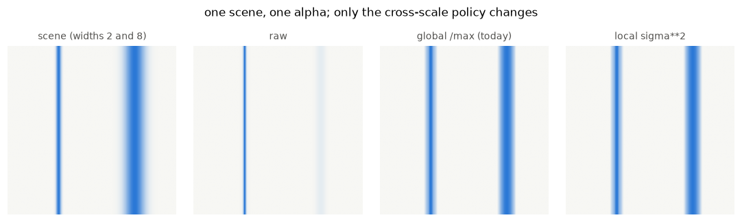

rows = []
for name, kw in POLICIES.items():
    out = fuse(SCENE, SIGMAS, **kw)
    _, won = detection_and_width(
        SCENE, SIGMAS, power=(0.0 if kw["scaling"] == "global" else 2 * kw["gamma"]))
    rows.append({
        "policy": name,
        "narrow value": round(float(out[MID, NARROW]), 4),
        "wide value": round(float(out[MID, WIDE]), 4),
        "wide / narrow": round(float(out[MID, WIDE] / out[MID, NARROW]), 3),
        "winning sigma at narrow": won[MID, NARROW],
        "winning sigma at wide": won[MID, WIDE],
    })
show_table(pd.DataFrame(rows).set_index("policy"))

Raw makes the narrow ridge win everywhere and the wide ridge score about 11 times weaker. The global /max makes both ridges 1.0 and puts the winning scale at 1 for both, so it carries no width information. The local $\sigma^2$ scores the two ridges within 1% of each other at a value below 1, and moves the winning scale with the width: 4 for the narrow ridge and the scan limit 8 for the wide.

4. The paper’s algorithm, and single-scale fidelity¶

The paper modifies the Hessian so that its eigenvalues flatten a second-order Gaussian filter along a ridge. In 2-D the flatness condition fixes $\alpha = -1/3$ , and the neuriteness is

\rho(x) = \begin{cases} \lambda(x)/\lambda_{\min} & \lambda(x) < 0,\\ 0 & \lambda(x) \ge 0, \end{cases}

(1)

with $\lambda$ the larger-magnitude modified eigenvalue and $\lambda_{\min}$ the smallest $\lambda$ over the whole image. The Gaussian scale $\sigma$ is a single tuning knob; Table 1 of the paper uses $\sigma = 2.0$ .

rho = paper_rho(RIDGE, SIGMA, alpha=-1 / 3)
nj = neuronj_magnitude(RIDGE, SIGMA, bright=True)
lam = selected_lambda(hessian_eigvals(RIDGE, SIGMA), -1 / 3)
paper_mag = np.where(lam < 0, -lam, 0.0)
lib_one = meijering(RIDGE, sigmas=[SIGMA], alpha=-1 / 3,
                    black_ridges=False, mode="nearest")

show_table(pd.DataFrame([
    {"pair": "paper rho vs NeuronJ / max",
     "max |difference|": f"{np.max(np.abs(rho - nj / nj.max())):.1e}"},
    {"pair": "NeuronJ magnitude vs paper |lambda|",
     "max |difference|": f"{np.max(np.abs(nj - paper_mag)):.1e}"},
    {"pair": "paper rho vs meijering, one sigma",
     "max |difference|": f"{np.max(np.abs(rho - lib_one)):.1e}"},
]))

The paper’s $\rho$ , the NeuronJ closed form, and meijering at one scale agree to numerical noise. The $\alpha$ sign does not show on a lone ridge, because /max hides it; it shows against a blob.

rows = []
for alpha in (-1 / 3, 1 / 3):
    lam_r = selected_lambda(hessian_eigvals(RIDGE, SIGMA), alpha)
    lam_b = selected_lambda(hessian_eigvals(BLOB, SIGMA), alpha)
    raw_r = -lam_r[MID, MID] if lam_r[MID, MID] < 0 else 0.0
    raw_b = -lam_b[MID, MID] if lam_b[MID, MID] < 0 else 0.0
    rows.append({"alpha": f"{alpha:+.4f}",
                 "ridge centre": f"{raw_r:.4f}",
                 "blob centre": f"{raw_b:.4f}",
                 "ridge / blob": f"{raw_r / max(raw_b, 1e-12):.3f}"})
show_table(pd.DataFrame(rows).set_index("alpha"))

Paper $\alpha = -1/3$ prefers the ridge; the shipped default $\alpha = +1/(2+1)$ prefers the blob. That defect is separate from the scale normalisation, and meijering_alpha.md carries it.

5. Scale normalisation: detection and width¶

5.1 The normalisation, from Lindeberg¶

A second derivative of a smoothed image falls with scale. Lindeberg normalises an order- $n$ derivative by $\sigma^{n\gamma}$ ; for a second derivative that is $\sigma^{2\gamma}$ . For a cylindrical Gaussian ridge of width $w$ , the cross-ridge second derivative on the axis is $e(\sigma) = w(w^2+\sigma^2)^{-3/2}$ . The normalised response $r_\gamma(\sigma) = \sigma^{2\gamma} e(\sigma)$ peaks at

\sigma^{*}(\gamma) = w\sqrt{\frac{2\gamma}{3-2\gamma}},

(2)

with value $D_\gamma = w^{2\gamma-2} c(\gamma)$ . Two cases matter:

$\gamma$	factor	winning scale	detection value
1	$\sigma^2$	$w\sqrt2$	0.3849, independent of $w$
$3/4$	$\sigma^{1.5}$	$w$	$\propto w^{-1/2}$

So $\sigma^2$ makes the detection value the same for every width, and $\sigma^{1.5}$ makes the winning scale equal the width but weakens wide ridges. Meijering et al. never fuse scales, so they never face the choice.

WIDTHS = np.array([1.0, 1.5, 2.0, 3.0, 4.0, 6.0, 8.0, 12.0])
GRID_G = np.linspace(0.02, 1.4, 400)

fig, axes = plt.subplots(1, 2, figsize=(9.6, 3.0))
axes[0].plot(GRID_G, np.sqrt(2 * GRID_G / (3 - 2 * GRID_G)), color=INK, lw=1.8)
axes[0].axhline(1.0, color=GRID, lw=1)
for gamma, colour, label in ((1.0, C_TWO, "1"), (0.75, C_ONE, "3/4")):
    axes[0].plot([gamma], [ridge_peak_sigma(1.0, gamma)], "o", color=colour,
                 ms=7, zorder=3)
    axes[0].annotate(f"gamma = {label}", (gamma, ridge_peak_sigma(1.0, gamma)),
                     textcoords="offset points", xytext=(6, -13), fontsize=8,
                     color=colour)
recede(axes[0], "winning scale against exponent")
axes[0].set_xlabel("gamma", fontsize=8, color=MUTED)
axes[0].set_ylabel("winning sigma / ridge width", fontsize=8, color=MUTED)

axes[1].loglog(WIDTHS, WIDTHS ** -2, "o-", color=MUTED, lw=1.6,
               label="raw  (gamma = 0)")
for gamma, colour, label in ((1.0, C_TWO, "sigma**2  (gamma = 1)"),
                             (0.75, C_ONE, "sigma**1.5  (gamma = 3/4)")):
    axes[1].loglog(WIDTHS, [ridge_peak_value(w, gamma) for w in WIDTHS],
                   "o-", color=colour, lw=1.8, label=label)
recede(axes[1], "detection value against ridge width")
axes[1].set_xlabel("ridge width w", fontsize=8, color=MUTED)
axes[1].set_ylabel("value at the winning scale", fontsize=8, color=MUTED)
axes[1].legend(frameon=False, fontsize=8)
fig.tight_layout()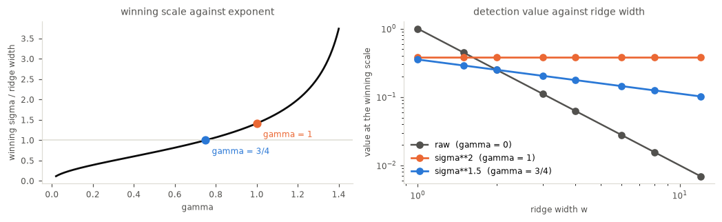

5.2 Detection map and width map¶

One scale scan gives two maps:

the detection map $D(x) = \max_\sigma r_\gamma(\sigma, x)$ ;
the width map $W(x) = \arg\max_\sigma r_\gamma(\sigma, x)$ .

meijering returns a detection map only, and its per-scale /max makes that a third normalisation again. A tapered ridge, whose width grows from 1.5 to 8 pixels, separates the maps.

HT, WT = 180, 220
tyy, txx = np.indices((HT, WT), dtype=float)
true_width = 1.5 + 6.5 * (tyy / (HT - 1))
tapered = np.exp(-((txx - WT / 2) ** 2) / (2 * true_width ** 2))
DENSE = np.array([1.0, 1.5, 2.0, 2.5, 3.0, 4.0, 5.0, 6.0, 7.0, 8.0, 9.0])

MAPS = {}
for gamma in (0.75, 1.0):
    det, win = detection_and_width(tapered, DENSE, power=2 * gamma)
    MAPS[gamma] = (det, np.where(det < 0.15 * det.max(), np.nan, win))

fig, axes = plt.subplots(2, 3, figsize=(11.5, 6.0))
bare(axes[0, 0], "input; true width grows downward")
axes[0, 0].imshow(tapered, cmap=SEQ)
for ax, gamma in zip(axes[0, 1:], (0.75, 1.0)):
    im = ax.imshow(MAPS[gamma][1], cmap="viridis", vmin=1, vmax=9)
    bare(ax, f"width map: gamma = {gamma:g}")
    fig.colorbar(im, ax=ax, fraction=0.046, label="winning sigma")
for ax, gamma in zip(axes[1, :2], (0.75, 1.0)):
    im = ax.imshow(MAPS[gamma][0], cmap=SEQ, vmin=0,
                   vmax=max(d.max() for d, _ in MAPS.values()))
    bare(ax, f"detection map: gamma = {gamma:g}")
    fig.colorbar(im, ax=ax, fraction=0.046)
axes[1, 2].plot(true_width[:, 0], np.arange(HT), color=INK, lw=1.8,
                label="true width")
for gamma, colour in ((0.75, C_ONE), (1.0, C_TWO)):
    axes[1, 2].plot(MAPS[gamma][1][:, WT // 2], np.arange(HT), color=colour,
                    lw=1.5, label=f"width map, gamma = {gamma:g}")
recede(axes[1, 2], "centreline: winning sigma against true width")
axes[1, 2].set_xlabel("sigma  (and true width)", fontsize=8, color=MUTED)
axes[1, 2].legend(frameon=False, fontsize=7)
fig.tight_layout()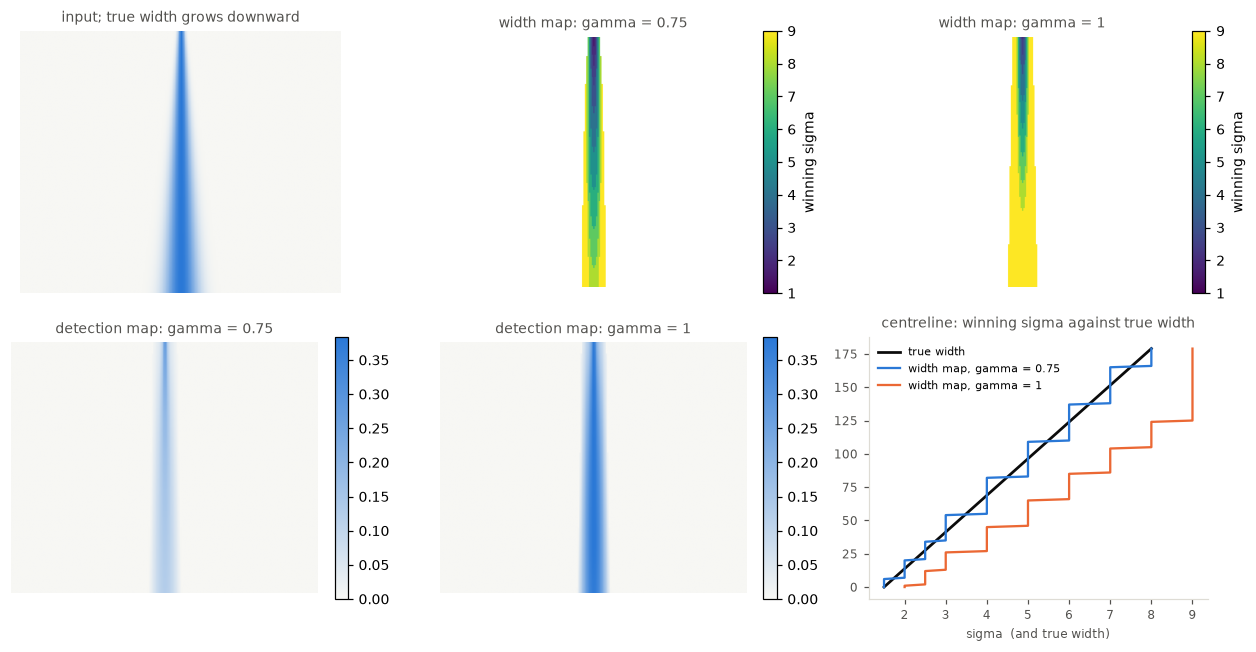

At $\gamma = 3/4$ the width map tracks the taper and the detection map fades as the ridge widens. At $\gamma = 1$ the width map sits above the taper (peaks at $w\sqrt2$ ) and the detection map stays bright. To read a width from the $\gamma = 1$ map, divide the winning scale by $\sqrt2$ .

5.3 The same statement on the filter¶

The closed forms are for an ideal ridge. On the discrete filter with its finite scan, the winning scale still moves with width under $\sigma^2$ , and the per-scale $\rho$ still drives every scale’s centre toward 1.

SCAN = (1.0, 2.0, 3.0, 5.0, 8.0)
rows = []
for w in (1.5, 3.0, 5.0, 8.0):
    img = gaussian_ridge(w)
    raw = [float(meijering_core(img, s)[MID, MID]) for s in SCAN]
    s2 = [float(meijering_core(img, s, power=2.0)[MID, MID]) for s in SCAN]
    rho_c = [float(paper_rho(img, s)[MID, MID]) for s in SCAN]
    rows.append({"width": w,
                 "argmax raw": SCAN[int(np.argmax(raw))],
                 "argmax sigma**2": SCAN[int(np.argmax(s2))],
                 "argmax per-sigma rho": SCAN[int(np.argmax(rho_c))]})
show_table(pd.DataFrame(rows).set_index("width"))

Raw strength peaks at the smallest $\sigma$ for every width. Per-scale $\rho$ also peaks there, because every scale’s centre is normalised toward 1. Only the $\sigma^2$ column moves with width.

6. Global or local normalisation¶

6.1 The two divisors agree at one scale¶

Write the bright-ridge response as $r = -\lambda$ where $\lambda < 0$ , and 0 elsewhere. The most negative $\lambda$ is the largest response, so $\lambda_{\min} = -\max r$ , and

\rho = \frac{\lambda}{\lambda_{\min}} = \frac{-r}{-\max r} = \frac{r}{\max r}.

(3)

So dividing by the paper’s $\lambda_{\min}$ and dividing by the library’s maximum are the same operation: both map the strongest response to 1 and the sign-selected background to 0. Both are global, so both are non-local. The two differ only in the multiscale case: the paper divides once, the library divides again at every scale.

lam = selected_lambda(hessian_eigvals(RIDGE, SIGMA), -1 / 3)
response = np.where(lam < 0, -lam, 0.0)
print(f"paper divisor   lambda_min      = {lam.min():.6f}")
print(f"library divisor -response.max() = {-response.max():.6f}")
print("paper rho equals meijering, one sigma: "
      f"{np.max(np.abs(paper_rho(RIDGE, SIGMA) - meijering(RIDGE, sigmas=[SIGMA], alpha=-1/3, black_ridges=False, mode='nearest'))):.1e}")

paper divisor   lambda_min      = -0.044721
library divisor -response.max() = -0.044721
paper rho equals meijering, one sigma: 0.0e+00

6.2 The per-scale maximum, and its cost¶

The per-scale /max is self-calibrating: it needs no contrast threshold and no scale exponent, and it corrects the gain the discrete operator actually has. Its costs are locality and strength. It is a whole-image statistic, so cropping or one bright pixel changes distant answers; and it pins each scale’s peak to 1, so “how strongly” is not comparable and the winning scale is a poor width cue. It also cancels any $\sigma$ power, because $\sigma^p$ is a positive per-scale factor.

wide8 = gaussian_ridge(8.0, n=201)
H = hessian_matrix(wide8, 4.0, mode="nearest", use_gaussian_derivatives=True)
lam8 = selected_lambda(hessian_matrix_eigvals(H), -1 / 3)
r8 = np.where(lam8 < 0, -lam8, 0.0)
per_scale = lambda a: a / a.max()
print("per-scale /max of r equals per-scale /max of 4**2 * r:",
      np.allclose(per_scale(r8), per_scale(4.0**2 * r8)))

per-scale /max of r equals per-scale /max of 4**2 * r: True

def far_change(before, after):
    """Largest change in the lower-right quadrant, as a fraction of its peak."""
    h, w = before.shape
    far = (slice(h // 2, None), slice(w // 2, None))
    return float(np.abs(before[far] - after[far]).max()
                 / max(np.abs(before[far]).max(), 1e-12))


edited = PHOTO.copy()
edited[:, 10:14] = 1.0  # a bright bar that can reset the global peak


rows = [
    {"method": "paper rho, sigma=2",
     "far max|delta|/peak": f"{far_change(paper_rho(PHOTO, 2), paper_rho(edited, 2)):.1%}"},
    {"method": "meijering, global /max",
     "far max|delta|/peak": f"{far_change(fuse(PHOTO, SIGMAS, scaling='global'), fuse(edited, SIGMAS, scaling='global')):.1%}"},
    {"method": "local sigma**2",
     "far max|delta|/peak": f"{far_change(fuse(PHOTO, SIGMAS, scaling='local'), fuse(edited, SIGMAS, scaling='local')):.1%}"},
    {"method": "sato (local)",
     "far max|delta|/peak": f"{far_change(sato(PHOTO, sigmas=SIGMAS, mode='nearest'), sato(edited, sigmas=SIGMAS, mode='nearest')):.1%}"},
]
show_table(pd.DataFrame(rows).set_index("method"))

The paper’s $\rho$ moves too: its divisor is global, like the library’s.

6.3 The option¶

The two policies answer different questions and cannot be combined, so the API should say which one it uses. A scale-explicit argument does that.

def meijering(image, sigmas=range(1, 10, 2), alpha=None,
              scaling="global", gamma=1.0, black_ridges=True,
              mode="reflect", cval=0):
    """scaling = 'global': divide each scale by its own maximum (current).
       scaling = 'local' : multiply the response by sigma ** (2 * gamma)."""

scaling="global" is today’s behaviour: a self-calibrated $[0,1]$ map, non-local, with no scale exponent, and weakest as a width cue. scaling="local", gamma=1 ( $\sigma^2$ ) is local and keeps absolute strength; it makes the detection value independent of ridge width (§5.1) and matches sato, ITK, DIPlib and the repaired frangi. scaling="local", gamma=0.75 ( $\sigma^{1.5}$ ) is the width estimator’s calibration. With one scale the option is inert, because the global divisor is then the paper’s own correction (§6.1).

7. How often, and how big¶

Three greyscale photographs from skimage.data, decimated so the longest side is about 200 px. The table reports the far-field change from a bright bar added near the edge, and the mean output ratio when the default global /max is replaced by local $\sigma^2$ .

def as_grey(image, target=200):
    """Greyscale float, decimated so the longest side is about `target`."""
    if image.ndim == 3:
        image = ski.color.rgb2gray(image)
    image = ski.util.img_as_float(image)
    step = max(1, max(image.shape) // target)
    return image[::step, ::step]


CORPUS = {"camera": as_grey(ski.data.camera()),
          "retina": as_grey(ski.data.retina()),
          "coins": as_grey(ski.data.coins())}

rows = []
for name, image in CORPUS.items():
    edit = image.copy()
    edit[:, 10:14] = 1.0
    glob = fuse(image, SIGMAS, scaling="global")
    glob_edit = fuse(edit, SIGMAS, scaling="global")
    loc = fuse(image, SIGMAS, scaling="local")
    rows.append({
        "image": name,
        "global far-field": f"{far_change(glob, glob_edit):.1%}",
        "local far-field": f"{far_change(loc, fuse(edit, SIGMAS, scaling='local')):.1%}",
        "mean local / mean global": round(float(loc.mean() / max(glob.mean(), 1e-12)), 3),
    })
show_table(pd.DataFrame(rows).set_index("image"))

Every image moves under the global /max and none moves under the local $\sigma^2$ . Replacing the default shrinks the mean output, by a factor between about 4 and 10 on this corpus, because the global /max pins each scale’s peak to 1 and $\sigma^2$ does not.

8. Properties that ought to hold¶

Each row is a promise, and the cell computes whether the current code keeps it. local is fuse(..., scaling="local") with $\gamma = 1$ .

def grey_level_change(fn, image, factor=10.0):
    """Relative change when the image is scaled by `factor`."""
    a, b = fn(image), fn(image * factor)
    return float(np.abs(a - b).max() / max(np.abs(a).max(), 1e-12))


edit = PHOTO.copy()
edit[:, 10:14] = 1.0
checks = [
    {"property": "single-scale rho equals paper",
     "value": f"{np.max(np.abs(paper_rho(RIDGE, SIGMA) - meijering(RIDGE, sigmas=[SIGMA], alpha=-1/3, black_ridges=False, mode='nearest'))):.1e}"},
    {"property": "NeuronJ agrees with the paper",
     "value": f"{np.max(np.abs(neuronj_magnitude(RIDGE, SIGMA) - np.where(selected_lambda(hessian_eigvals(RIDGE, SIGMA), -1/3) < 0, -selected_lambda(hessian_eigvals(RIDGE, SIGMA), -1/3), 0.0))):.1e}"},
    {"property": "global /max is grey-level invariant",
     "value": f"{grey_level_change(lambda im: fuse(im, SIGMAS, scaling='global'), PHOTO):.1e}"},
    {"property": "local sigma**2 is not grey-level invariant",
     "value": f"{grey_level_change(lambda im: fuse(im, SIGMAS, scaling='local'), PHOTO):.1e}"},
    {"property": "global /max is non-local (far field)",
     "value": f"{far_change(fuse(PHOTO, SIGMAS, scaling='global'), fuse(edit, SIGMAS, scaling='global')):.1%}"},
    {"property": "local sigma**2 is local (far field)",
     "value": f"{far_change(fuse(PHOTO, SIGMAS, scaling='local'), fuse(edit, SIGMAS, scaling='local')):.1%}"},
]
show_table(pd.DataFrame(checks).set_index("property"))

The local policy breaks grey-level invariance on purpose: it keeps absolute strength, so scaling the image scales the answer. The global /max keeps grey-level invariance and pays for it with non-locality.

9. Comparators¶

NeuronJ is the authors’ implementation and the fair check for algorithm fidelity. meijering at one scale reproduces it. The other libraries have no Meijering neuriteness; the comparable choice is their scale policy.

nj_mag = neuronj_magnitude(RIDGE, SIGMA, bright=True)
paper_mag = np.where(
    selected_lambda(hessian_eigvals(RIDGE, SIGMA), -1 / 3) < 0,
    -selected_lambda(hessian_eigvals(RIDGE, SIGMA), -1 / 3), 0.0)
show_table(pd.DataFrame([
    {"comparator": "NeuronJ Costs.run (alpha = -1/3)",
     "metric": "vs paper |lambda| where lambda < 0",
     "value": f"{np.max(np.abs(nj_mag - paper_mag)):.1e}"},
    {"comparator": "skimage meijering(sigmas=[sigma])",
     "metric": "vs paper rho",
     "value": f"{np.max(np.abs(meijering(RIDGE, sigmas=[SIGMA], alpha=-1/3, black_ridges=False, mode='nearest') - paper_rho(RIDGE, SIGMA))):.1e}"},
]))

software	Meijering neuriteness?	scales	scale policy
NeuronJ (authors)	Yes	single $\sigma$	global display normalisation; no fusion
MATLAB `meij_hessianeigs`	modified Hessian only	single $\sigma$	$\sigma^2$ on the kernels; caller fuses
ITK / SimpleITK	no named Meijering	multiscale objectness	local $\sigma^2$ ; returns a width map separately
DIPlib	no (Frangi vesselness)	single scale	$\sigma^2$ plus a supremum is a caller recipe
sato (in scikit-image)	no	multiscale	local $\sigma^2$
skimage `frangi` (`frangi-fixes`)	no	multiscale	local $\sigma^2$ on the Hessian norm
skimage `meijering`	yes	multiscale	grid written below

The rows are read from source or documentation, except sato, which runs in §6. No sibling divides by a per-scale image statistic except meijering and Jerman’s MATLAB. ITK is the one that returns a width map, and it returns it as a separate output rather than by retuning the detection exponent.

10. Ways forward¶

Each candidate is a runnable cell. The fuse helper already implements them; the figure shows the same two-width scene under the three policies, and the table gives the detection value and winning scale.

fig, axes = plt.subplots(1, 3, figsize=(9.0, 3.0))
for ax, (name, kw) in zip(axes, POLICIES.items()):
    out = fuse(SCENE, SIGMAS, **kw)
    im = ax.imshow(out, cmap=SEQ, vmin=0, vmax=out.max())
    bare(ax, name)
    fig.colorbar(im, ax=ax, fraction=0.046)
fig.suptitle("candidate cross-scale policies on the two-width scene", y=1.03)
fig.tight_layout()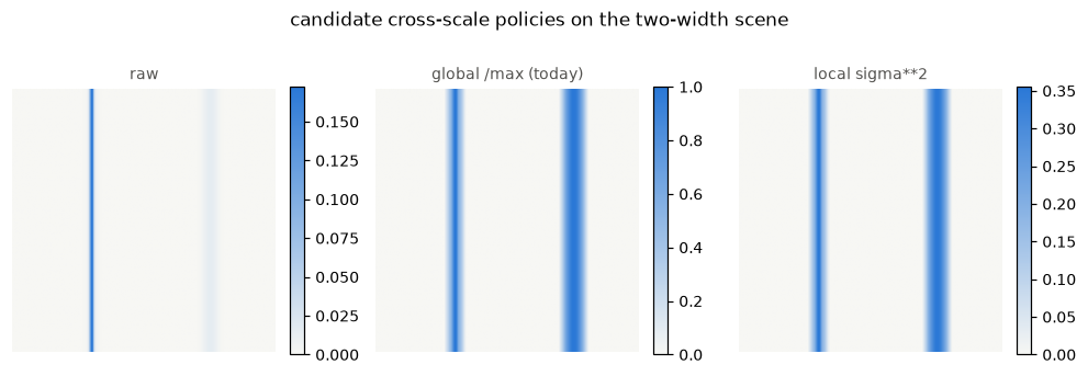

rows = []
for name, kw in POLICIES.items():
    out = fuse(SCENE, SIGMAS, **kw)
    power = 0.0 if kw["scaling"] == "global" else 2 * kw["gamma"]
    _, won = detection_and_width(SCENE, SIGMAS, power=power)
    rows.append({
        "policy": name,
        "narrow value": round(float(out[MID, NARROW]), 4),
        "wide value": round(float(out[MID, WIDE]), 4),
        "wide / narrow": round(float(out[MID, WIDE] / out[MID, NARROW]), 3),
        "winning sigma at narrow": won[MID, NARROW],
        "winning sigma at wide": won[MID, WIDE],
    })
show_table(pd.DataFrame(rows).set_index("policy"))

For a detection map, the local $\sigma^2$ is the candidate: it keeps a value below 1, makes the two widths score alike, and stays local. For a width map, $\sigma^{1.5}$ makes the winning scale equal the width. The global /max is neither: it makes both values 1 and leaves the winning scale uninformative about width.

11. What each fix costs¶

The three policies share the Hessian work, so the time cost is small. The output change is the real cost: replacing the default with local $\sigma^2$ changes almost every pixel and no longer spans $[0,1]$ .

import time

costs = []
for name, kw in POLICIES.items():
    started = time.perf_counter()
    for _ in range(3):
        out = fuse(PHOTO, SIGMAS, **kw)
    costs.append({
        "policy": name,
        "seconds": round((time.perf_counter() - started) / 3, 3),
        "output max": round(float(out.max()), 3),
        "max |diff| vs global": f"{np.abs(out - fuse(PHOTO, SIGMAS, scaling='global')).max():.3g}",
    })
show_table(pd.DataFrame(costs).set_index("policy"))

The local $\sigma^2$ changes the photograph by up to 0.8 on the global $[0,1]$ scale, and lowers the maximum from 1.0 to 0.36. Single-scale calls do not change, because the option is inert at one scale (§6.1). No policy is slower than another beyond measurement noise; the loop cost is the per-scale Hessian.

12. What not to do¶

Do not add $\sigma^2$ on top of the per-scale /max. The /max cancels any positive per-scale factor (§6.2), so the sum is the /max again.

Do not read a width from the per-scale /max. Pinning each scale’s peak to 1 removes the absolute differences that carry width information (§5.3).

Do not treat the paper’s $\lambda_{\min}$ as a licence for a per-scale divisor. The paper divides once, at one scale (§6.1). Applying the same correction at every scale before a maximum is the extension that #6436 left open, and #6446 chose without a paper basis.

Do not call a local patch normalisation “what the paper does”. The paper’s normalisation is global (§6.3).

13. Summary¶

question	answer
Does skimage match the paper?	At one $\sigma$ with $\alpha=-1/3$ and bright-ridge polarity, yes (§4). The defaults do not: the $\alpha$ sign and the multiscale `/max` both differ.
Was the paper single-scale?	Yes. Table 1 uses $\sigma=2.0$ and the text says the detector is tuned to a specific width; NeuronJ exposes one scale.
Scaling across $\sigma$	The paper defines none. A local $\sigma$ power calibrates the winning scale: $\gamma=1$ gives a flat detection value at $w\sqrt2$ ; $\gamma=3/4$ gives the width but weakens wide ridges by $w^{-1/2}$ (§5.1).
Detection vs width	One scan gives a detection map and a width map. `meijering` returns a detection map only. Detecting wide structures favours $\gamma=1$ ; reading width favours $\gamma=3/4$ (§5.2).
Global vs local	At one scale the paper’s $\lambda_{\min}$ and the library’s maximum are the same divisor (§6.1). Applying it at every scale is what breaks locality and strength; it also cancels any $\sigma$ power (§6.2).
How often	Every corpus image moves under the global `/max` and none moves under local $\sigma^2$ (§7).
Comparators	NeuronJ agrees with the paper at one scale; the sibling filters use a local $\sigma^2$ and ITK also returns a width map (§9).
Recommendation	Expose `scaling=“global”

Limits. Synthetic Gaussian ridges and blobs, and three skimage.data photographs decimated to about 200 px; Hessian from the Gaussian-derivative path (use_gaussian_derivatives=True); the paper’s Table 1 images are not available, so fidelity is checked against the paper’s formula and the NeuronJ closed form, not against its figures. ITK, DIPlib and OpenCV have no Meijering $\rho$ to compare, so §9 compares their scale policy from source, not their output. The $\alpha$ mechanics live in meijering_alpha.md; the $\gamma$ calibration follows Lindeberg (1998) §5.6.1.

print(f"scikit-image {ski.__version__}")

scikit-image 0.26.1rc0.dev0

References¶

Meijering, E., Jacob, M., Sarria, J. ‐C. F., Steiner, P., Hirling, H., & Unser, M. (2004). Design and validation of a tool for neurite tracing and analysis in fluorescence microscopy images. Cytometry Part A, 58A(2), 167–176. 10.1002/cyto.a.20022