The second derivative of a smoothed image

skimage.feature.hessian_matrix computes second derivatives of an image at a chosen scale. Four filters depend on it — frangi, sato, meijering and hessian — and it has been through three implementations in as many years.

This is a review of how it works, why it was built the way it was, and what a better version would look like. It builds up from the problem rather than from the code, and every claim is measured against a standard fixed before any method is judged.

on_hessian.md is the diagnostic companion: it goes further into each defect and carries the candidate fixes in full. This document is the argument.

Coordinates are in array order throughout: the first index runs down the picture, the second runs right.

import numpy as np
import pandas as pd
import scipy.ndimage as ndi
import matplotlib.pyplot as plt
from matplotlib.colors import LinearSegmentedColormap, TwoSlopeNorm
from scipy.signal import resample

from IPython.display import Markdown, display

from nbhelper import show_table

import skimage as ski
from skimage.feature import hessian_matrix
from skimage.filters import frangi, sato, meijering, hessian

fatal: not a git repository (or any of the parent directories): .git
fatal: not a git repository (or any of the parent directories): .git

# Slots 1 to 3 of the reference categorical palette, validated all-pairs.
C_ONE, C_TWO, C_THREE = "#2a78d6", "#eb6834", "#1baf7a"
INK, MUTED, GRID = "#0b0b0b", "#52514e", "#dedcd5"
SEQ = LinearSegmentedColormap.from_list("seq", ["#f7f7f4", C_ONE])
DIV = LinearSegmentedColormap.from_list("div", [C_ONE, "#f2f1ec", C_TWO])

plt.rcParams.update(
    {"figure.dpi": 110, "font.size": 9, "axes.titlesize": 9,
     "axes.titlecolor": MUTED, "figure.facecolor": "white"}
)


def show(ax, data, title=None, diverging=False):
    if diverging:
        limit = np.abs(data).max() or 1.0
        image = ax.imshow(data, cmap=DIV, norm=TwoSlopeNorm(0, -limit, limit))
    else:
        image = ax.imshow(data, cmap=SEQ)
    ax.set_xticks([]); ax.set_yticks([])
    for spine in ax.spines.values():
        spine.set_visible(False)
    if title:
        ax.set_title(title)
    return image


def recede(ax, title=None):
    ax.tick_params(labelsize=8, colors=MUTED)
    for spine in ("top", "right"):
        ax.spines[spine].set_visible(False)
    for spine in ("left", "bottom"):
        ax.spines[spine].set_color(GRID)
    if title:
        ax.set_title(title)
    return ax

1. The problem¶

An image is a grid of numbers. A derivative is a limit over distances that go to zero. The grid has no values between its samples, so the derivative of an image is not defined until we say what we mean by it.

Differencing neighbouring pixels is the obvious answer and a bad one: it amplifies noise without limit, and the answer changes if the same scene is photographed at a different resolution. The standard remedy is to fix a scale. Convolve with a Gaussian of width sigma, which is smooth and differentiable, and differentiate that instead. The scale is then part of the question rather than an accident of the sensor.

For second derivatives this gives the Hessian at scale sigma: for a 2-D image, three distinct entries, because mixed partials are equal.

    H = | Hii  Hij |          Hij = d2/di dj  ( G_sigma * f )
        | Hij  Hjj |

Its eigenvalues describe local curvature. At each pixel the Hessian is a symmetric 2×2 matrix, so it has two real eigenvalues λ and two orthogonal eigenvectors. Each eigenvalue is the second directional derivative of the smoothed image along its eigenvector: how sharply the intensity bends when you step in that direction. The eigenvectors are the principal-curvature axes — the directions of strongest and weakest bend.

Sign and magnitude both matter. For a bright structure on a dark background, curvature toward the structure is negative (the intensity has a local maximum along that axis). Two large negative eigenvalues mean the surface bends down in every direction — a blob. One large negative eigenvalue and one near zero mean it bends across a line but is flat along it — a ridge. That is the basis of ridge detection, which is what frangi, sato and meijering do.

from skimage.feature import hessian_matrix_eigvals

# One grid and one closed-form toolkit for every Gaussian test image below.
# A single blob (`SOLO`) and a single ridge are special cases of the same
# machinery as the multi-Gaussian `SCENE` (§3.3) — not a second analytic path.
SCENE_N = 201
SCENE_MARGIN = 50
SCENE_INTERIOR = slice(SCENE_MARGIN, -SCENE_MARGIN)
BLOB_S, RIDGE_W = 4.0, 3.0
centre = SCENE_N // 2
si, sj = np.indices((SCENE_N, SCENE_N), dtype=float)
crop = SCENE_INTERIOR


def blob_image(center, width, weight=1.0):
    """Unit-integral isotropic Gaussian, times `weight`."""
    ci, cj = center
    r2 = (si - ci) ** 2 + (sj - cj) ** 2
    return weight * np.exp(-r2 / (2 * width**2)) / (2 * np.pi * width**2)


def ridge_image(axis, center, width, weight=1.0):
    """Unit-integral 1-D Gaussian along `axis` (0 = rows, 1 = columns)."""
    coord = si if axis == 0 else sj
    return weight * np.exp(-((coord - center) ** 2) / (2 * width**2)) / (
        np.sqrt(2 * np.pi) * width)


def blob_hessian(center, width, sigma, weight=1.0):
    """Closed-form Hessian of a smoothed isotropic blob."""
    t2 = width**2 + sigma**2
    ci, cj = center
    di, dj = si - ci, sj - cj
    g = weight * np.exp(-(di**2 + dj**2) / (2 * t2)) / (2 * np.pi * t2)
    return [g * (di**2 / t2**2 - 1 / t2),
            g * (di * dj / t2**2),
            g * (dj**2 / t2**2 - 1 / t2)]


def ridge_hessian(axis, center, width, sigma, weight=1.0):
    """Closed-form Hessian of a smoothed axis-aligned ridge."""
    t2 = width**2 + sigma**2
    coord = si if axis == 0 else sj
    d = coord - center
    g = weight * np.exp(-(d**2) / (2 * t2)) / (np.sqrt(2 * np.pi * t2))
    curv = g * (d**2 / t2**2 - 1 / t2)
    zero = np.zeros_like(g)
    if axis == 0:                                 # varies along rows
        return [curv, zero, zero]
    return [zero, zero, curv]                     # varies along columns


def render_scene(parts):
    """Sum the continuous pieces onto the integer grid."""
    image = np.zeros((SCENE_N, SCENE_N), dtype=float)
    for part in parts:
        if part["kind"] == "blob":
            image += blob_image(part["center"], part["width"], part["weight"])
        else:
            image += ridge_image(part["axis"], part["center"],
                                 part["width"], part["weight"])
    return image


def analytic_scene_hessian(parts, sigma):
    """Exact Hessian of the smoothed scene, term by term (the analytic standard).

    "Analytic" here always means this closed form: each Gaussian stays a
    Gaussian under smoothing (`t**2 = s**2 + sigma**2`), differentiated by
    hand — no discrete filter, DCT, or supersampling.
    """
    acc = [np.zeros((SCENE_N, SCENE_N)),
           np.zeros((SCENE_N, SCENE_N)),
           np.zeros((SCENE_N, SCENE_N))]
    for part in parts:
        if part["kind"] == "blob":
            terms = blob_hessian(part["center"], part["width"],
                                 sigma, part["weight"])
        else:
            terms = ridge_hessian(part["axis"], part["center"],
                                  part["width"], sigma, part["weight"])
        for a, t in zip(acc, terms):
            a += t
    return acc


SOLO = ({"kind": "blob", "center": (centre, centre),
         "width": BLOB_S, "weight": 1.0},)
solo = render_scene(SOLO)

# Vertical bright ridge: curved across columns, flat along rows.
RIDGE = ({"kind": "ridge", "axis": 1, "center": centre,
          "width": RIDGE_W, "weight": 1.0},)
ridge = render_scene(RIDGE)


def eig_pair(image, sigma=2.0):
    """Stronger and weaker principal curvatures, by |λ|.

    `hessian_matrix_eigvals` returns eigenvalues in ascending algebraic order
    (most negative first). Here we re-sort by magnitude so the panels compare
    curvature *strength*, and the sign on each panel still shows bright vs dark.
    """
    elems = hessian_matrix(image, sigma=sigma, mode="nearest",
                           use_gaussian_derivatives=True)
    eigs = hessian_matrix_eigvals(elems)
    order = np.argsort(np.abs(eigs), axis=0)
    by_mag = np.take_along_axis(eigs, order, axis=0)
    return by_mag[1], by_mag[0]                  # λ_strong, λ_weak


fig, axes = plt.subplots(2, 3, figsize=(9.0, 5.4))
for row, (image, label) in enumerate(((solo, "blob"), (ridge, "ridge"))):
    strong, weak = eig_pair(image)
    show(axes[row, 0], image[crop, crop], label)
    show(axes[row, 1], strong[crop, crop], r"$\lambda$ stronger $|\cdot|$",
         diverging=True)
    show(axes[row, 2], weak[crop, crop], r"$\lambda$ weaker $|\cdot|$",
         diverging=True)
    # Centre values: concrete numbers for the pattern the eye should see.
    axes[row, 0].text(
        0.02, 0.05,
        f"centre:  λ_strong = {strong[centre, centre]:+.4f}\n"
        f"         λ_weak   = {weak[centre, centre]:+.4f}",
        transform=axes[row, 0].transAxes, fontsize=7, color=INK,
        family="monospace",
        bbox=dict(boxstyle="round,pad=0.25", facecolor="white", edgecolor=GRID),
    )

axes[0, 0].set_ylabel("both λ large and negative\n→ blob",
                      fontsize=8, color=MUTED)
axes[1, 0].set_ylabel("one large negative, one ≈ 0\n→ ridge",
                      fontsize=8, color=MUTED)
fig.suptitle("principal curvatures λ at sigma = 2 "
             "(negative = bright ridge/blob on dark)",
             y=1.02)
fig.tight_layout()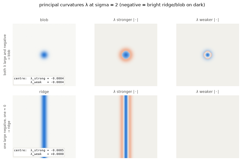

On the blob the two centre values are equal and negative: isotropic downward bend. On the ridge the strong eigenvalue is negative (bend across the line) and the weak one is ~0 (no bend along it). Blue in the maps is that negative curvature; the weak panel for the ridge is nearly blank because there is almost nothing to show.

The three Hessian entries themselves are the second derivatives that those eigenvalues are built from:

entries = hessian_matrix(solo, sigma=2.0, mode="nearest",
                         use_gaussian_derivatives=True)

fig, axes = plt.subplots(1, 4, figsize=(10.0, 2.6))
show(axes[0], solo[crop, crop], "a blob (SOLO)")
for ax, name, entry in zip(axes[1:], ("Hii", "Hij", "Hjj"), entries):
    show(ax, entry[crop, crop], name, diverging=True)
fig.suptitle("the same blob: its three second derivatives at sigma = 2", y=1.04)
fig.tight_layout()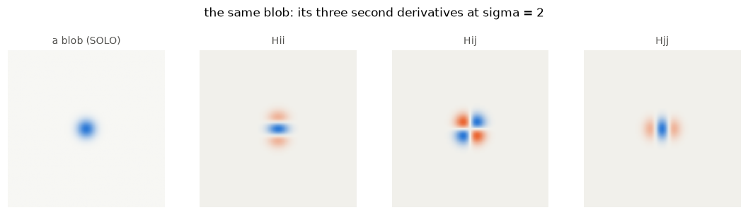

So the quantity we are after is fixed and unambiguous: the second derivative of the image after smoothing by a Gaussian of width sigma. The rest of this document is about how to compute that quantity on a discrete grid, and how to tell whether a given method has computed it correctly.

2. Two ways to compute it¶

Convolution and differentiation commute. For a Gaussian G and an image f:

    d/dx ( G * f )  ==  ( dG/dx ) * f

Either side is a route to the same continuous quantity, and the two sides suggest two different programs.

Route A — smooth, then difference. Take the left-hand side literally. Blur the image, then apply a numerical derivative to the blurred result. The derivative can be the simplest central difference; the blurring has already done the work of making that safe.

Route B — differentiate the Gaussian. Take the right-hand side. Build a kernel that is already the second derivative of a Gaussian and convolve once. No differencing step exists to be inaccurate.

def route_a(image, sigma, mode="nearest"):
    """Smooth, then difference: the left-hand side, literally."""
    smoothed = ndi.gaussian_filter(image, sigma, mode=mode)
    d_i, d_j = np.gradient(smoothed)
    d_ii, d_ij = np.gradient(d_i)
    _, d_jj = np.gradient(d_j)
    return [d_ii, d_ij, d_jj]


def route_b(image, sigma, mode="nearest"):
    """Convolve once with a derivative-of-Gaussian kernel: the right-hand side."""
    return [ndi.gaussian_filter(image, sigma, order=order, mode=mode)
            for order in ([2, 0], [1, 1], [0, 2])]

Both are a few lines, both return something plausible, and at a comfortable scale they agree.

a, b = route_a(solo, 2.0), route_b(solo, 2.0)
scale = max(np.abs(e).max() for e in b)
worst = max(np.abs(x - y).max() for x, y in zip(a, b))
print(f"route A against route B at sigma = 2: worst difference "
      f"{worst / scale:.2%} of the peak response")

route A against route B at sigma = 2: worst difference 4.85% of the peak response

A few per cent apart. Which of them is closer to the answer? Nothing so far can say — the two routes only disagree with each other. That needs a third thing.

3. A standard to judge them by¶

Two approximations that differ tell you only that at least one is wrong. To say which, we need a reference computed a third way, decided before any method is put on trial.

There are four available, and they check each other.

3.1 A closed form, for images made of Gaussians¶

A Gaussian smoothed by a Gaussian is another Gaussian, with t**2 = s**2 + sigma**2. So for a test image built from Gaussians, the smoothed Hessian is known exactly, in closed form, with no discretisation anywhere. That is what analytic_scene_hessian computes (§1): term-by-term for every blob or ridge in a scene. SOLO is the one-blob case; SCENE below adds widths and ridges. Tables that say “vs analytic” mean against this closed form — not against dct_hessian or gold_hessian.

def error_against(computed, truth, region=SCENE_INTERIOR):
    """Worst disagreement over the three entries, on a shared interior."""
    scale = max(np.abs(e).max() for e in truth)
    return max(np.abs(a[region, region] - b[region, region]).max()
               for a, b in zip(computed, truth)) / scale

This is exact but narrow: it holds only for images we construct, and a method could in principle do well on a smooth Gaussian and badly on a photograph. The multi-Gaussian SCENE widens the test without leaving the closed form.

3.2 Supersampling, for any image¶

The second standard removes that limitation and costs a great deal.

Treat the image as samples of a continuous function — which is the assumption that makes “the derivative of an image” mean anything at all. Reconstruct that function on a grid k times finer, where the sampling is k times denser and so the discretisation error is k-fold smaller. Do the differentiation there, at scale k * sigma in fine-grid units. Then return to the original grid.

The reconstruction is band-limited resampling, which is the interpolation consistent with that same assumption. A second derivative with respect to coarse coordinates is k**2 times the derivative with respect to fine ones, which is the only scaling involved.

from concurrent.futures import ThreadPoolExecutor


def upsample(image, factor):
    """Band-limited resampling onto a `factor` times finer grid."""
    finer = resample(image, image.shape[0] * factor, axis=0)
    return resample(finer, image.shape[1] * factor, axis=1)


# `gold_hessian` on a 256² photograph at factor=4 builds a 2048² grid and runs
# three Gaussian filters there (~seconds each). Later cells ask for the same
# (image, sigma, factor, mode) many times; cache the fine grid (shared across
# sigmas) and the finished tensors so repeats are free.
_GOLD_FINE = {}
_GOLD_HESSIAN = {}


def _array_key(image):
    """Content key for cache lookups (shape + digest; images are small here)."""
    return (image.shape, image.dtype.str, hash(image.tobytes()))


def gold_hessian(image, sigma, factor=4, mode="nearest"):
    """The reference: differentiate where the sampling error is negligible.

    Pad once, resample finer, take the derivative at `factor * sigma`, decimate,
    crop. Costs `factor**2` in memory and time, which is why it is a yardstick
    and not an implementation.

    `mode` must match the method under test. A reference that extends the image
    by a different rule measures that difference and calls it an error.
    """
    image = np.asarray(image)
    cache_key = (_array_key(image), float(sigma), int(factor), mode)
    cached = _GOLD_HESSIAN.get(cache_key)
    if cached is not None:
        return cached

    # `ndimage` and `numpy.pad` spell the same rules differently.
    pad_mode = {"nearest": "edge", "reflect": "symmetric", "mirror": "reflect",
                "wrap": "wrap", "constant": "constant"}[mode]
    # `resample` reconstructs from the DFT, so it reads its input as periodic.
    # The padded array is a whole number of periods only when each axis is
    # padded by half its length; any other amount leaves a wrap-around step,
    # and the ringing from that is a floor `factor` cannot lower.
    pads = [n // 2 for n in image.shape]
    if min(pads) < 8 * sigma + 2:
        raise ValueError("image too small at this sigma: the kernel would "
                         "reach the crop")

    fine_key = (_array_key(image), int(factor), mode)
    fine_hit = _GOLD_FINE.get(fine_key)
    if fine_hit is None:
        fine = upsample(np.pad(image, [(p, p) for p in pads], mode=pad_mode),
                        factor)
        _GOLD_FINE[fine_key] = (fine, pads)
    else:
        fine, pads = fine_hit

    orders = ([2, 0], [1, 1], [0, 2])
    sigma_fine = factor * sigma

    def _one(order):
        return ndi.gaussian_filter(fine, sigma_fine, order=order, mode=mode,
                                   truncate=8)

    # The three orders are independent; ndimage releases the GIL in C.
    with ThreadPoolExecutor(max_workers=3) as pool:
        elems = list(pool.map(_one, orders))
    coarse = [(e[::factor, ::factor] * factor**2) for e in elems]
    result = [e[pads[0]:-pads[0], pads[1]:-pads[1]] for e in coarse]
    _GOLD_HESSIAN[cache_key] = result
    return result

Three details in that function are not decoration. The image is padded once, before anything else happens, so the boundary rule is applied a single time — any reference that extends the image more than once is measuring its own artefacts. The padding clears the kernel, so the crop never sees an edge. And the pad is half the image on each axis rather than a multiple of sigma, because the resampler reads its input as periodic: that is the amount which makes the padded array a whole number of periods.

The fine-grid derivatives still use SciPy’s uncorrected order=2 kernels; at factor * sigma those kernels are already well sampled (section 5), so the yardstick is not carrying the small-sigma leak it is used to judge.

The reference therefore has two error sources, and only one of them answers to factor. Refinement controls how well the fine-grid kernels are sampled. Reconstruction — whether the padded array really is periodic — does not move with factor at all, so a convergence check in factor alone cannot see it. Section 3.6 measures both against an image whose exact answer is known.

3.3 The two standards agree¶

The supersampled reference is only worth having if it converges to the answer we already know. On a multi-Gaussian scene the closed form still applies, and it stresses several widths and ridge geometry at once — not only a single blob that has already decayed before it reaches the border.

SCENE = (
    {"kind": "blob", "center": (70, 70), "width": 2.0, "weight": 1.0},
    {"kind": "blob", "center": (70, 130), "width": 3.5, "weight": 1.2},
    {"kind": "blob", "center": (130, 70), "width": 5.0, "weight": 0.8},
    {"kind": "blob", "center": (130, 130), "width": 7.0, "weight": 1.0},
    {"kind": "ridge", "axis": 1, "center": 100, "width": 2.5, "weight": 0.6},
    {"kind": "ridge", "axis": 0, "center": 100, "width": 4.0, "weight": 0.5},
)
scene = render_scene(SCENE)

factors = (1, 2, 4, 8)
rows = []
for sigma in (0.3, 0.4, 0.5, 0.7, 1.0, 2.0):
    truth = analytic_scene_hessian(SCENE, sigma)
    row = {"sigma": sigma}
    for k in factors:
        err = error_against(gold_hessian(scene, sigma, factor=k), truth)
        row[f"k = {k}"] = f"{err:.3%}"
    rows.append(row)
show_table(pd.DataFrame(rows))

At k = 4 the reference reproduces the closed form to the printed precision at comfortable scales, and refining further changes nothing. So k = 4 is enough on this scene. (Below sigma ≈ 1 the gap is the small-σ kernel sampling of section 5, not a failure of the closed form.)

It is tempting to read that as trustworthiness on images with no closed form, and that step does not follow. Convergence in k tests one of the two things that can go wrong — how well the fine-grid kernels are sampled — and a sum of Gaussians well inside the margin is still a weak probe of padding, because the signal has decayed before the border where reconstruction acts. Section 3.6 puts the same reference on an image that does reach the border and finds an error k cannot touch.

The k = 1 column is worth a second look, because it is not a reference at all: it is route B computed directly on the original grid, with no refinement. At sigma = 0.3 it is wrong by a large factor. That is the first sign of the problem section 5 is about, and it appears here as a control rather than as a claim.

3.4 A gallery of Gaussians, still closed form¶

SCENE in §3.3 is already the widened closed-form test: several blob widths plus axis-aligned ridges, all inside SCENE_MARGIN so the border never enters the interior score. The Hessian is linear, and each term stays closed form under smoothing — the same analytic_scene_hessian used for SOLO.

The left panel below is the input that hessian_matrix will see. The other two are not approximations: they are the algebra evaluated on the grid. Narrow structures dominate $H$ at this scale; the wide blob at bottom-right is already mild.

fig, axes = plt.subplots(1, 3, figsize=(10.5, 3.2))
show(axes[0], scene, "collection (blobs + ridges)")
show(axes[1], analytic_scene_hessian(SCENE, 2.0)[0],
     r"analytic $H_{ii}$ at $\sigma = 2$", diverging=True)
show(axes[2], analytic_scene_hessian(SCENE, 2.0)[2],
     r"analytic $H_{jj}$ at $\sigma = 2$", diverging=True)
fig.suptitle("closed-form Hessian on a multi-Gaussian scene "
             f"(margin {SCENE_MARGIN} px)", y=1.04)
fig.tight_layout()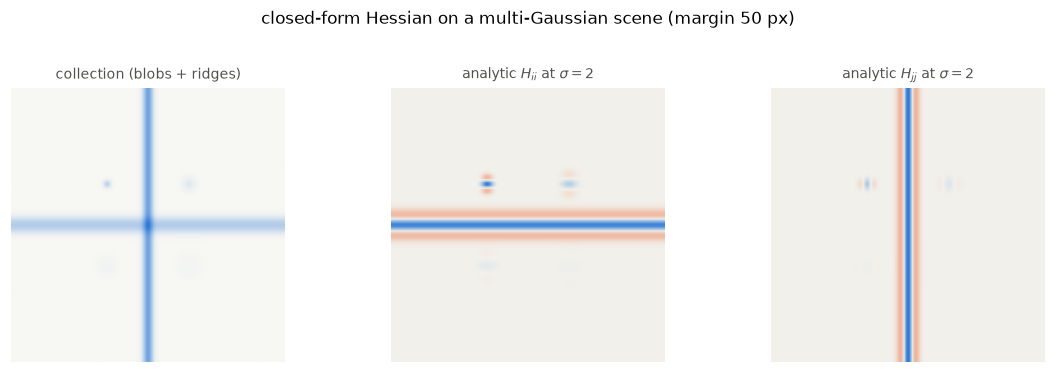

A few more layouts, so the construction is clearly a family rather than one picture.

VARIANTS = {
    "blobs only": (
        {"kind": "blob", "center": (70, 80), "width": 2.0, "weight": 1.0},
        {"kind": "blob", "center": (100, 120), "width": 4.0, "weight": 1.0},
        {"kind": "blob", "center": (140, 90), "width": 6.5, "weight": 1.0},
    ),
    "ridges only": (
        {"kind": "ridge", "axis": 1, "center": 80, "width": 2.0, "weight": 0.8},
        {"kind": "ridge", "axis": 1, "center": 120, "width": 5.0, "weight": 0.8},
        {"kind": "ridge", "axis": 0, "center": 100, "width": 3.0, "weight": 0.6},
    ),
    "mixed, unequal weights": (
        {"kind": "blob", "center": (90, 90), "width": 3.0, "weight": 2.0},
        {"kind": "blob", "center": (120, 140), "width": 8.0, "weight": 0.4},
        {"kind": "ridge", "axis": 0, "center": 70, "width": 2.5, "weight": 1.0},
        {"kind": "ridge", "axis": 1, "center": 150, "width": 4.0, "weight": 0.7},
    ),
}

fig, axes = plt.subplots(1, 3, figsize=(10.5, 3.2))
for ax, (name, parts) in zip(axes, VARIANTS.items()):
    show(ax, render_scene(parts), name)
fig.suptitle("other placements: still a sum of Gaussians inside the margin",
             y=1.04)
fig.tight_layout()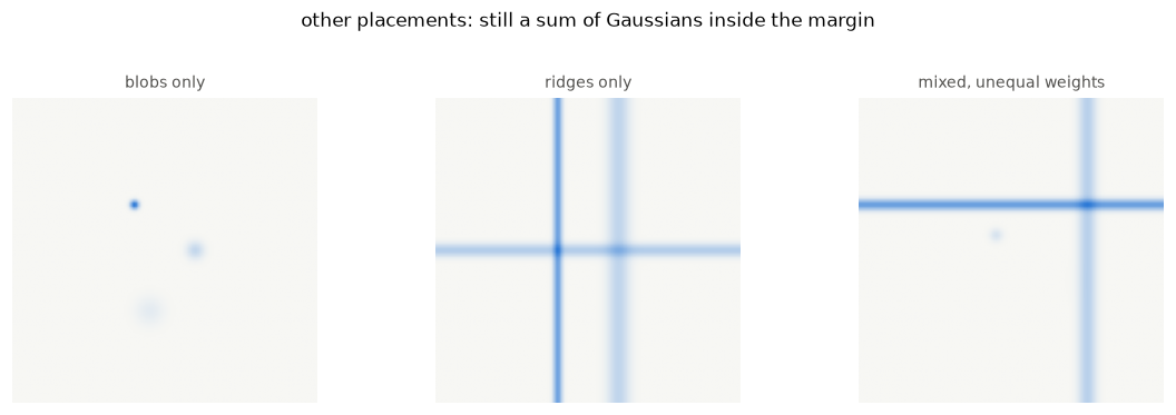

3.5 How the four standards relate¶

Two checks for the closed form and the supersampler. The fourth standard — the DCT continuous Gaussian — follows in §3.6.

Band-limited sampling tracks the multi-Gaussian analytic. §3.3 already showed gold_hessian approaching analytic_scene_hessian(SCENE, ·) as k rises. At the working refinement, compare gold and the shipped filter to that same analytic on the interior.

# At the working refinement, multi-analytic vs gold, and vs the shipped filter.
rows = []
for sigma in (0.7, 1.0, 1.5, 2.0, 3.0):
    truth = analytic_scene_hessian(SCENE, sigma)
    gold = gold_hessian(scene, sigma, factor=4)
    shipped = hessian_matrix(scene, sigma=sigma, mode="nearest",
                             use_gaussian_derivatives=True)
    rows.append({
        "sigma": sigma,
        "gold k=4 vs analytic":
            f"{error_against(gold, truth):.3%}",
        "shipped vs analytic":
            f"{error_against(shipped, truth):.3%}",
        "shipped vs gold k=4":
            f"{error_against(shipped, gold):.3%}",
    })
show_table(pd.DataFrame(rows))

What each standard is for. The Gaussian closed form (analytic_scene_hessian) is an identity on images we construct — SOLO for one blob, SCENE for mixed widths and ridges — and is the only yardstick that does not assume a band-limited interpolant. The DCT continuous gold (§3.6) is the band-limited exact answer for an arbitrary image under half-sample reflection. The supersampler is what remains when the pad mode must match the code under test (nearest, and so on). On Gaussian scenes these are not competing opinions: the closed forms are identities, and both numerical standards converge to them on the interior.

At sigma ≥ 1.5 the shipped filter, the supersampler, and the multi-Gaussian analytic agree to the printed precision on the interior. Below that they part company — and the analytic, not the supersampler, is the one that stays exact, which is why the gallery earns its keep next to the supersampler.

3.6 DCT continuous Gaussian (IPOL 2016)¶

The supersampler approximates continuous convolution by refining the grid. Rey-Otero and Delbracio (IPOL 2016) do the continuous convolution exactly under a stated interpolant (their Algorithm 2): type-II DCT of the $M\times N$ image, weight each coefficient by $\exp\!\bigl(-\tfrac12\sigma^2(\omega_m^2+\omega_n^2)\bigr)$ with $\omega_m = \pi m/M$ , $\omega_n = \pi n/N$ , and invert. Equivalently — their §2.2 — DFT of the half-sample even extension of size $2M\times 2N$ , $\breve u_{k,l} = u_{s_M(k),s_N(l)}$ with $s_M(k)=\min(k,2M-1-k)$ , then the same Gaussian weights at frequencies $2\pi m/(2M)=\pi m/M$ . That is continuous Gaussian smoothing of a trigonometric polynomial — no factor, no sampled $G''$ kernel.

The paper stops at the smoothed field. The Hessian below is the same continuous field differentiated: multiply by $-\omega_i\omega_j$ before the inverse transform. Pure second derivatives stay in the DCT cosine basis; the mixed term needs the sine–sine (DST) partner, so the DFT-of-extension form is the convenient one that yields all three entries together.

The extension repeats the edge sample ([a,b,c,c,b,a]). That is SciPy / scikit-image mode='reflect', not mirror (whole-sample, no edge repeat).

def mirror_symmetrize(image):
    """Half-sample even extension of IPOL 2016 §2.2 / Algorithm 2."""
    M, N = image.shape
    ii = np.minimum(np.arange(2 * M), 2 * M - 1 - np.arange(2 * M))
    jj = np.minimum(np.arange(2 * N), 2 * N - 1 - np.arange(2 * N))
    return image[np.ix_(ii, jj)]


def dct_hessian(image, sigma):
    """Hessian of the IPOL DCT-Gaussian continuous scale-space.

    Exact continuous $G_\\sigma * u$ under the DCT interpolant (IPOL Algorithm
    2), then exact second derivatives of that field. Boundary model is
    half-sample reflection (`mode='reflect'`), not `nearest` or `mirror`.
    """
    M, N = image.shape
    ext = mirror_symmetrize(image)
    freqs_i = np.fft.fftfreq(ext.shape[0]) * 2 * np.pi
    freqs_j = np.fft.fftfreq(ext.shape[1]) * 2 * np.pi
    wi, wj = np.meshgrid(freqs_i, freqs_j, indexing="ij")
    Fg = np.fft.fft2(ext) * np.exp(-0.5 * sigma**2 * (wi**2 + wj**2))
    return [np.fft.ifft2(Fg * (-wi**2)).real[:M, :N],
            np.fft.ifft2(Fg * (-wi * wj)).real[:M, :N],
            np.fft.ifft2(Fg * (-wj**2)).real[:M, :N]]

On SOLO or SCENE, DCT is not an approximation of the Gaussian closed form on the interior we score — it is that form to floating point — because a Gaussian well inside the frame is unchanged by the even extension there. The table uses SCENE, the stricter case (several widths and ridges).

rows = []
for sigma in (0.5, 0.7, 1.0, 2.0):
    truth = analytic_scene_hessian(SCENE, sigma)
    rows.append({
        "sigma": sigma,
        "dct vs analytic":
            f"{error_against(dct_hessian(scene, sigma), truth):.2e}",
        "gold k=4 vs analytic":
            f"{error_against(gold_hessian(scene, sigma, factor=4), truth):.3%}",
        "gold k=4 vs dct":
            f"{error_against(gold_hessian(scene, sigma, factor=4), dct_hessian(scene, sigma)):.3%}",
    })
show_table(pd.DataFrame(rows))

DCT matches the term-by-term analytic; the supersampler only catches up once k is large enough that SciPy’s kernels are well sampled.

Those two tables are agreement on images built from Gaussians, and a Gaussian decays to nothing at the frame edge. That is the one shape for which the supersampler’s padding cannot misbehave, so the tables above cannot separate the two references. A test that can: a single DCT-II basis function, which is exactly band-limited, so the model both references assume is not an approximation but a fact, and whose smoothed Hessian is known in closed form.

For $u_{k,l} = \cos a(k+\tfrac12)\cos b(l+\tfrac12)$ with $a = \pi m/M$ , $b = \pi n/N$ , smoothing multiplies by $E = e^{-\sigma^2(a^2+b^2)/2}$ and

\partial_{xx} = -a^2 E u, \qquad \partial_{xy} = ab\,E \sin a(k+\tfrac12)\sin b(l+\tfrac12), \qquad \partial_{yy} = -b^2 E u .

(1)

BAND_N = 128
bk, bl = np.indices((BAND_N, BAND_N), dtype=float)


def band_limited(m, n, sigma):
    """A DCT-II basis image, and the exact Hessian of its smoothing."""
    a, b = np.pi * m / BAND_N, np.pi * n / BAND_N
    ca, cb = np.cos(a * (bk + 0.5)), np.cos(b * (bl + 0.5))
    u = ca * cb
    damp = np.exp(-0.5 * sigma**2 * (a**2 + b**2))
    return u, [-a * a * damp * u,
               a * b * damp * np.sin(a * (bk + 0.5)) * np.sin(b * (bl + 0.5)),
               -b * b * damp * u]


BAND_INTERIOR = slice(30, -30)
rows = []
for m, n in ((8, 12), (48, 32), (100, 90), (120, 118)):
    for sigma in (0.5, 1.0):
        u, truth = band_limited(m, n, sigma)
        rows.append({
            "m, n": f"({m}, {n})",
            "freq / Nyquist": f"{max(m, n) / BAND_N:.2f}",
            "sigma": sigma,
            "dct": f"{error_against(dct_hessian(u, sigma), truth, BAND_INTERIOR):.1e}",
            "gold k=4": f"{error_against(gold_hessian(u, sigma, factor=4, mode='reflect'), truth, BAND_INTERIOR):.1e}",
            "gold k=8": f"{error_against(gold_hessian(u, sigma, factor=8, mode='reflect'), truth, BAND_INTERIOR):.1e}",
        })
show_table(pd.DataFrame(rows))

Both are exact at every frequency, to 10^-12 or better at 94% of Nyquist. That is the validation the Gaussian tables could not give: the two references share a model but no code — one weights transform coefficients, the other reconstructs on a finer grid and differentiates with sampled kernels — and they agree with a closed form neither was built from.

What makes the supersampler exact here is the periodic padding of section 3.2, and that is worth demonstrating rather than asserting, because the obvious choice of pad is not periodic. Pad just enough to clear the kernel and the reference develops an error that refinement cannot touch.

def gold_with_pad(image, sigma, factor, pad, mode="reflect"):
    """`gold_hessian` with the pad forced, to isolate the reconstruction error."""
    fine = upsample(np.pad(image, pad, mode="symmetric"), factor)
    elems = [ndi.gaussian_filter(fine, factor * sigma, order=order, mode=mode,
                                 truncate=8)
             for order in ([2, 0], [1, 1], [0, 2])]
    return [(e[::factor, ::factor] * factor**2)[pad:-pad, pad:-pad]
            for e in elems]


u, truth = band_limited(120, 118, 1.0)          # 0.94 of Nyquist
scan = {"vary factor, pad = 10":
            {f"factor={k}": f"{error_against(gold_with_pad(u, 1.0, k, 10), truth, BAND_INTERIOR):.1e}"
             for k in (2, 4, 8, 16)},
        "vary pad, factor = 4":
            {f"pad={p}": f"{error_against(gold_with_pad(u, 1.0, 4, p), truth, BAND_INTERIOR):.1e}"
             for p in (10, 20, 96, BAND_N // 2, BAND_N)}}
show_table(pd.DataFrame(scan["vary factor, pad = 10"], index=["error"]))
show_table(pd.DataFrame(scan["vary pad, factor = 4"], index=["error"]))

Four refinements, one number: at a pad of 10 the error sits at $8\times10^{-3}$ whether the grid is refined twice or sixteen times. Then the pad moves it by ten orders of magnitude — and pad = 96 is worse than pad = 64, so this is not a matter of padding more. resample reconstructs from the DFT, so it reads its input as periodic; only a pad of half the image, or a whole multiple of that, makes the padded array a whole number of periods of the symmetric extension. Half the image is the smallest that works, and is what section 3.2 uses. With it, the supersampler and the DCT agree to floating point on a photograph too.

# The photograph of section 6, brought forward: a real image is the case the
# a single smooth Gaussian cannot stand in for.
CAMERA = ski.util.img_as_float(ski.data.camera())[::2, ::2]

rows = []
for sigma in (0.5, 1.0, 2.0):
    rows.append({
        "sigma": sigma,
        "gold k=4 vs dct, camera interior":
            f"{error_against(gold_hessian(CAMERA, sigma, factor=4, mode='reflect'), dct_hessian(CAMERA, sigma), slice(40, -40)):.1e}",
    })
show_table(pd.DataFrame(rows))

That agreement is the real validation of both. They are built on the same band-limited model but share no code: one reconstructs on a finer grid and differentiates with sampled kernels, the other weights coefficients in a transform. Agreeing to 10^-14 on a photograph is evidence neither is carrying an artefact of its own.

When to use which. dct_hessian is the primary standard. It is exact rather than convergent, it has no refinement parameter whose adequacy has to be argued, it satisfies the semi-group property to machine precision — which is the criterion Rey-Otero and Delbracio use — and it costs one pair of transforms instead of factor**2 of everything. Use it for every interior score, at any mode, and for border scores when the method under test uses mode='reflect'.

gold_hessian is kept for the one thing the DCT cannot do: score the border under a boundary rule that is not half-sample reflection. hessian_matrix itself defaults to mode='constant', and the methods compared in sections 6 to 8 run at mode='nearest', so that is not a hypothetical — section 8 is entirely supersampler work. For images built as sums of Gaussians the closed form of §3.1 / §3.3 remains the simplest exact answer, and is the only one of the three that does not assume the image is band-limited.

That last point is worth keeping in view. The DCT and the supersampler are not independent: both model the image as a trigonometric polynomial, so their agreement is a check on implementation, not on the model. The closed form is what tests the model, and it only exists for images we construct. On a photograph the band-limited assumption is an assumption, and no measurement in this notebook can discharge it.

4. Why the library moved from differences to Gaussian derivatives¶

With a standard in hand the two routes of section 2 can be judged rather than compared.

SCALES = (0.4, 0.5, 0.7, 1.0, 1.5, 2.0, 3.0, 5.0)

rows = []
for sigma in SCALES:
    # Interior score: DCT matches the Gaussian analytic on SOLO (§3.6).
    truth = dct_hessian(solo, sigma)
    rows.append({
        "sigma": sigma,
        "route A, differences": f"{error_against(route_a(solo, sigma), truth):.2%}",
        "route B, Gaussian": f"{error_against(route_b(solo, sigma), truth):.2%}",
    })
show_table(pd.DataFrame(rows))

Route A sits on a floor of a few per cent that no amount of smoothing removes. Route B is a tenth of a per cent out above sigma = 1 — fifty times better — and falls apart below it, by four orders of magnitude.

The floor has a clean explanation. np.gradient uses the central difference (f[n+1] - f[n-1]) / 2, whose frequency response is i sin(w) where the true derivative’s is i w. Applying it twice gives -sin(w)**2 against -w**2. The ratio sin(w)**2 / w**2 is 1 only at w = 0 and falls away everywhere else, so the operator under-reports curvature at every frequency the image actually contains.

w = np.linspace(1e-6, np.pi, 400)

fig, ax = plt.subplots(figsize=(5.6, 2.8))
ax.plot(w, np.sin(w) ** 2 / w**2, color=C_TWO, lw=2,
        label="central difference, twice")
ax.axhline(1.0, color=INK, lw=2, label="exact second derivative")
ax.set_xlabel("spatial frequency, radians per pixel", fontsize=8, color=MUTED)
ax.set_ylabel("gain, relative to exact", fontsize=8, color=MUTED)
recede(ax, "why differencing has a floor")
ax.legend(frameon=False, fontsize=8)
fig.tight_layout()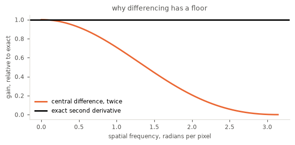

Smoothing more does not help, because smoothing changes what the image contains, not what the operator does to it: the shortfall at each frequency is fixed. That is why route A’s column is flat.

This is the case for the switch, and hessian_matrix has a use_gaussian_derivatives argument that makes it, with a FutureWarning announcing that route B will become the default. Above sigma = 1 the argument is unanswerable — route B is within a tenth of a percent where route A is wrong by 2 to 5%, a gap of nearly two orders of magnitude that does not close at any scale.

Route B’s residual is not zero, and it is worth saying why it now shows. The standard here is the DCT, which shares no machinery with either route. The supersampled reference would have flattered route B, because it computes its own fine-grid derivatives with the same SciPy kernels route B uses on the coarse grid, so part of route B’s error is present in that reference too and cancels. An independent standard does not cancel it. The number is small either way; the point is that a reference built from the method under test cannot measure the method under test.

Below sigma = 1 it reverses, and badly. That is the next section.

5. The two-pass solution, and why it was chosen¶

The naive form of route B is to ask SciPy for a second-order derivative directly, order=[2, 0]. Doing so fails at small sigma in a way that is easy to see and hard to argue with: the operator responds to an image with no structure at all. A second derivative must return 0 on a constant and 1 on r**2 / 2:

flat = np.ones((40, 40))
ramp = np.repeat((np.arange(400.0)[:, None] - 200) ** 2 / 2, 8, axis=1)

rows = []
for sigma in (0.5, 0.7, 1.0, 1.5):
    on_flat = ndi.gaussian_filter(flat, sigma, order=[2, 0], mode="nearest")[20, 20]
    on_ramp = ndi.gaussian_filter(ramp, sigma, order=[2, 0], mode="nearest")[200, 4]
    rows.append({"sigma": sigma, "constant": on_flat, "quadratic": on_ramp})
show_table(pd.DataFrame(rows), floatfmt=".4f")

At sigma = 0.5 a flat field reads as curvature of -0.56. The cause is sampling: the kernel is built by evaluating the continuous second derivative of a Gaussian on the integer grid, and at half a pixel wide that formula swings through its whole range between one sample and the next. The positive flanks no longer cancel the negative well, so the coefficients do not sum to zero, and a kernel that does not sum to zero responds to constants.

In one dimension the failure is two moment conditions that any discrete second derivative must meet:

    sum(k)             ==  0        no response to a constant
    sum(k * x**2) / 2  ==  1        exact on f = x**2 / 2

At small sigma the sampled G’’ breaks both.

def sampled_g2(sigma, truncate=8):
    """1-D second derivative of a Gaussian, sampled on the integer grid."""
    reach = int(truncate * sigma + 0.5)
    x = np.arange(-reach, reach + 1, dtype=float)
    g = np.exp(-(x**2) / (2 * sigma**2))
    g /= g.sum()
    return x, g * ((x**2 - sigma**2) / sigma**4)


def apply_1d(signal, kernel):
    return ndi.correlate1d(signal, kernel, mode="nearest")


# Domain wide enough that edge effects sit outside the plotted window.
x = np.arange(-80, 81, dtype=float)
constant = np.ones_like(x)
quadratic = x**2 / 2
mid = 80
win_c = slice(mid - 8, mid + 9)               # |x| <= 8
win_q = slice(mid - 4, mid + 5)               # |x| <= 4; keeps the bow in view

fig, axes = plt.subplots(3, 3, figsize=(9.6, 7.2),
                         gridspec_kw={"height_ratios": [1.1, 1, 1]})
for col, sigma in enumerate((0.5, 1.0, 1.5)):
    kx, k = sampled_g2(sigma)
    m0, m2 = k.sum(), (k * kx**2).sum() / 2
    resp_c = apply_1d(constant, k)
    resp_q = apply_1d(quadratic, k)

    axes[0, col].stem(kx, k, linefmt=C_TWO, markerfmt="o", basefmt=" ")
    axes[0, col].axhline(0, color=GRID, lw=1)
    axes[0, col].set_xlim(-8, 8)
    recede(axes[0, col], f"sampled G'', σ = {sigma:g}")
    axes[0, col].text(
        0.98, 0.95,
        f"Σk = {m0:+.3f}\nΣkx²/2 = {m2:.3f}",
        transform=axes[0, col].transAxes, ha="right", va="top",
        fontsize=7, family="monospace", color=INK,
        bbox=dict(boxstyle="round,pad=0.2", facecolor="white", edgecolor=GRID),
    )

    axes[1, col].plot(x[win_c], constant[win_c], color=MUTED, lw=1.2,
                      label="f = 1")
    axes[1, col].plot(x[win_c], resp_c[win_c], color=C_TWO, lw=2,
                      label="k * f")
    axes[1, col].axhline(0, color=INK, lw=1, ls="--", label="required: 0")
    recede(axes[1, col], "zeroth moment: response to a constant")
    axes[1, col].set_ylim(-1.0, 0.3)

    # Near the origin the quadratic response should be the flat line 1.
    # A non-zero Σk mixes in a multiple of x²/2 and bows the curve.
    axes[2, col].plot(x[win_q], resp_q[win_q], color=C_TWO, lw=2,
                      label="k * (x²/2)")
    axes[2, col].axhline(1, color=INK, lw=1, ls="--", label="required: 1")
    axes[2, col].axhline(m2, color=C_ONE, lw=1, ls=":",
                         label=f"Σkx²/2 = {m2:.2f}")
    recede(axes[2, col], "second moment: response to x²/2")
    axes[2, col].set_ylim(-2.0, 2.0)
    axes[2, col].set_xlabel("x", fontsize=8, color=MUTED)

axes[1, 0].legend(frameon=False, fontsize=7, loc="lower left")
axes[2, 0].legend(frameon=False, fontsize=7, loc="lower left")
axes[0, 0].set_ylabel("coefficient", fontsize=8, color=MUTED)
axes[1, 0].set_ylabel("amplitude", fontsize=8, color=MUTED)
axes[2, 0].set_ylabel("amplitude", fontsize=8, color=MUTED)
fig.suptitle("1-D moment failures of the sampled second-derivative kernel",
             y=1.01)
fig.tight_layout()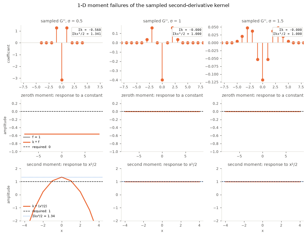

At sigma = 0.5 the kernel sums to −0.56, so a constant comes back as that same number (middle row). The second moment is 1.34 instead of 1, and the non-zero sum also folds a multiple of x²/2 into the response, so the bottom row bows instead of sitting on the dashed line at 1. By sigma = 1.5 both moments are already right to the printed precision. The 2-D picture is the same zeroth-moment leak, drawn as an image:

# The leak is not a scalar curiosity: it paints a non-zero field onto a blank.
flat_big = np.ones((64, 64))
naive_flat = ndi.gaussian_filter(flat_big, 0.5, order=[2, 0], mode="nearest")

fig, axes = plt.subplots(1, 2, figsize=(6.4, 2.8))
show(axes[0], flat_big, "constant image")
im = show(axes[1], naive_flat, "order=[2, 0] at sigma = 0.5", diverging=True)
fig.colorbar(im, ax=axes[1], fraction=0.046)
fig.suptitle("a kernel that does not sum to zero responds to nothing", y=1.04)
fig.tight_layout()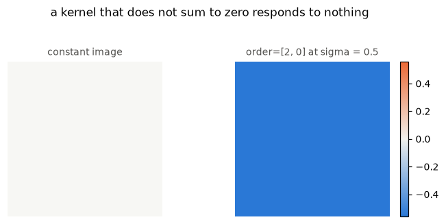

This was reported in 2021 as Are scipy second-order Gaussian derivatives correct?, by someone who met it on an image that was constant down every column and got 1e-5 where zero was the only right answer.

The fix scikit-image adopted is in the same question. Rather than ask for a second derivative, ask for a first derivative twice. The source records the decision:

    # Apply two successive first order Gaussian derivative operations, as
    # detailed in:
    # https://dsp.stackexchange.com/questions/78280/are-scipy-second-order-gaussian-derivatives-correct

It works, and for a reason worth stating plainly: a first-derivative kernel is odd, k[-n] == -k[n], so its coefficients cancel in pairs and it sums to zero by symmetry no matter how coarsely it is sampled. Composing two of them never asks SciPy for the even kernel that leaks. Each pass uses sigma / sqrt(2), because two Gaussians of that width compose to one of width sigma.

def two_pass(image, sigma, mode="nearest"):
    """The shipped scheme: two first-order passes at sigma / sqrt(2)."""
    scaled = sigma / np.sqrt(2)
    kwargs = dict(mode=mode, truncate=8 if sigma > 1 else 100)
    grad_i = ndi.gaussian_filter(image, scaled, order=[1, 0], **kwargs)
    grad_j = ndi.gaussian_filter(image, scaled, order=[0, 1], **kwargs)
    return [ndi.gaussian_filter(grad_i, scaled, order=[1, 0], **kwargs),
            ndi.gaussian_filter(grad_i, scaled, order=[0, 1], **kwargs),
            ndi.gaussian_filter(grad_j, scaled, order=[0, 1], **kwargs)]


print("the same two tests, two-pass")
rows = []
for sigma in (0.5, 0.7, 1.0, 1.5):
    rows.append({
        "sigma": sigma,
        "constant": two_pass(flat, sigma)[0][20, 20],
        "quadratic": two_pass(ramp, sigma)[0][200, 4],
    })
show_table(pd.DataFrame(rows), floatfmt=".4f")

the same two tests, two-pass

The response to a constant is now exactly zero at every scale, which is what the change was for. The quadratic column shows what it cost: at sigma = 0.5 the scheme reports 8% of the curvature that is there. The leak is gone and the gain has collapsed in its place.

The same source carries one more decision, and it is worth quoting because its reasoning is checkable:

    # For small sigma, the SciPy Gaussian filter suffers from aliasing and edge
    # artifacts, given that the filter will approximate a sinc or sinc
    # derivative which only goes to 0 very slowly (order 1/n**2). Thus, we use
    # a much larger truncate value to reduce any edge artifacts.
    truncate = 8 if all(s > 1 for s in sigma) else 100

The diagnosis is right and the remedy does not follow from it. A sampled Gaussian derivative decays like a Gaussian, not like a sinc, so the far taps a wide window keeps are not small-but-helpful — they are zero, and the moments a narrow window gets wrong a wide one gets wrong identically. (The shipped guard applies to the first-order passes at sigma / sqrt(2); the second-derivative taps below make the same point more directly, because that is the kernel whose leak the two-pass scheme was written to avoid.)

def taps(sigma, order, truncate):
    """The 1-D kernel `gaussian_filter` builds, from the explicit formula."""
    reach = int(truncate * sigma + 0.5)
    x = np.arange(-reach, reach + 1).astype(float)
    g = np.exp(-(x**2) / (2 * sigma**2))
    g /= g.sum()
    if order == 0:
        return x, g
    if order == 1:
        return x, g * (x / sigma**2)
    return x, g * ((x**2 - sigma**2) / sigma**4)


x_wide, k_wide = taps(0.5, 2, 100)
mid = k_wide.size // 2
peak = np.abs(k_wide).max()
show_table(pd.DataFrame([
    {"n": n,
     "|k[n]| / peak": abs(k_wide[mid + n]) / peak,
     "1/n**2": 1.0 / n**2}
    for n in (1, 2, 4, 8)
]), floatfmt=".1e")

x_narrow, k_narrow = taps(0.5, 2, 8)
show_table(pd.DataFrame([
    {"truncate": 8, "sum of taps": f"{k_narrow.sum():+.4f}"},
    {"truncate": 100, "sum of taps": f"{k_wide.sum():+.4f}"},
]))

# Same support, same leak: widening the window does not restore sum(k) = 0.
fig, ax = plt.subplots(figsize=(6.0, 2.8))
ax.plot(x_narrow, k_narrow, color=C_TWO, lw=2, marker="o", ms=4,
        label=f"truncate = 8,  sum = {k_narrow.sum():+.3f}")
ax.plot(x_wide, k_wide, color=C_ONE, lw=1.2, alpha=0.7,
        label=f"truncate = 100, sum = {k_wide.sum():+.3f}")
ax.axhline(0, color=GRID, lw=1)
ax.set_xlim(-8, 8)
ax.set_xlabel("tap index", fontsize=8, color=MUTED)
ax.set_ylabel("coefficient", fontsize=8, color=MUTED)
recede(ax, "sampled G'' at sigma = 0.5: the far taps are already zero")
ax.legend(frameon=False, fontsize=8)
fig.tight_layout()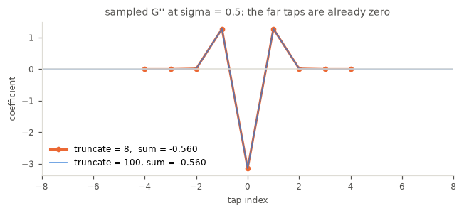

Fifty-two orders of magnitude apart at n = 8, and the two sums are identical. truncate = 100 buys nothing and costs a great deal, because every reference and every padded construction downstream has to clear a hundred-pixel radius rather than eight. Section 7 removes the reason for it.

6. The two-pass solution against the standard¶

The scheme is what hessian_matrix ships today. Measured against the standard, it is good in the interior above sigma = 1, and it has two faults that the tests in section 5 could not see.

PHOTO = ski.util.img_as_float(ski.data.camera())[::2, ::2]


def border_and_interior(method, image, sigma, margin=20):
    """Worst disagreement with the standard, at the border and away from it."""
    truth = gold_hessian(image, sigma)
    got = method(image, sigma)
    scale = max(np.abs(e).max() for e in truth)
    inner = (slice(margin, -margin),) * 2
    return (max(np.abs(a - b).max() for a, b in zip(got, truth)) / scale,
            max(np.abs(a[inner] - b[inner]).max() for a, b in zip(got, truth)) / scale)


rows = []
for sigma in (0.5, 1.0, 1.5, 3.0):
    whole, inner = border_and_interior(two_pass, PHOTO, sigma)
    rows.append({
        "sigma": sigma,
        "worst anywhere": f"{whole:.1%}",
        "interior only": f"{inner:.1%}",
    })
show_table(pd.DataFrame(rows))

The first fault is at the border, and it does not shrink with sigma. From sigma = 1.5 upwards the interior is exact and the border is still about a fifth of the peak wrong — roughly 19% at sigma = 1.5 and 3, of the same order at larger scales.

sigma = 1.5
truth = gold_hessian(PHOTO, sigma)
gap = np.abs(two_pass(PHOTO, sigma)[1] - truth[1])

fig, axes = plt.subplots(1, 3, figsize=(9.6, 2.8))
show(axes[0], truth[1], "standard, mixed element", diverging=True)
show(axes[1], two_pass(PHOTO, sigma)[1], "two-pass, mixed element", diverging=True)
im = show(axes[2], gap, "|two-pass − standard|")
fig.colorbar(im, ax=axes[2], fraction=0.046)
fig.suptitle(f"the disagreement is a border band (sigma = {sigma})", y=1.04)
fig.tight_layout()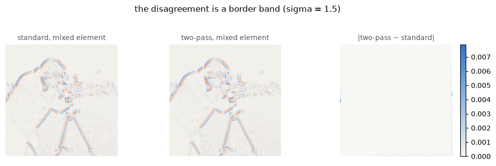

The cause is that the scheme makes two calls, and each call applies the boundary rule for itself. mode says how to continue the image past its edge. The first pass consumes the image and produces a derivative field; the second pass then applies the same rule to that, as though a smoothed derivative continued the way the image does. It does not. Outside the image the derivative field keeps varying for about a kernel radius before it settles, and the second call asserts it is constant from the edge onwards.

A single call is exact, because a boundary extension along one axis commutes with filtering along a different axis. It is only filtering the same axis twice that goes wrong.

one_pass_1d = lambda a, axis: ndi.gaussian_filter1d(a, 1.5, axis=axis, mode="nearest")


def against_pad_once(f, image, pad=40):
    big = np.pad(image, pad, mode="edge")
    return np.abs(f(image) - f(big)[pad:-pad, pad:-pad]).max()


show_table(pd.DataFrame([
    {"composition": label, "error vs pad-once": against_pad_once(f, PHOTO)}
    for label, f in (
        ("one pass, axis 0", lambda a: one_pass_1d(a, 0)),
        ("axis 0 then axis 1, different axes",
         lambda a: one_pass_1d(one_pass_1d(a, 0), 1)),
        ("axis 0 twice, the same axis",
         lambda a: one_pass_1d(one_pass_1d(a, 0), 0)),
    )
]), floatfmt=".2e")

The second fault follows from the first. Because the mixed element is built by differentiating along one axis and then the other, the answer depends on which axis went first — and hessian_matrix exposes exactly that choice through its order argument. The two orders are meant to be the same tensor relabelled.

rc = hessian_matrix(PHOTO, sigma=1.5, mode="nearest", order="rc",
                    use_gaussian_derivatives=True)
xy = hessian_matrix(PHOTO, sigma=1.5, mode="nearest", order="xy",
                    use_gaussian_derivatives=True)
scale = max(np.abs(e).max() for e in rc)
gap = max(np.abs(a - b).max() for a, b in zip(rc, xy[::-1])) / scale
print(f"order='rc' against order='xy', same quantity: {gap:.1%} of the peak")

order='rc' against order='xy', same quantity: 11.3% of the peak

# The mixed element under both labellings: disagreement sits at the border.
fig, axes = plt.subplots(1, 3, figsize=(9.6, 2.8))
show(axes[0], rc[1], "order='rc', Hij", diverging=True)
show(axes[1], xy[1], "order='xy', Hxy ≡ Hij", diverging=True)
im = show(axes[2], np.abs(rc[1] - xy[1]), "|rc − xy| on the mixed element")
fig.colorbar(im, ax=axes[2], fraction=0.046)
fig.suptitle("a labelling parameter that changes the answer by 11%", y=1.04)
fig.tight_layout()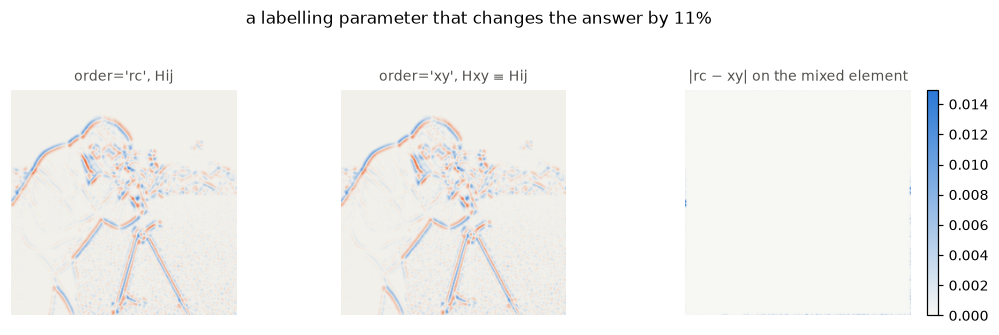

Eleven per cent apart on this photograph, for a parameter documented as choosing between two labellings of one answer. Neither is right: both are approximations that disagree at the border, and the standard says so. The figure depends on the image — on uniform random data it reaches 40% — because it is driven by how much structure sits near the edge.

7. One pass, with corrected kernels¶

The border fault has an obvious remedy once the cause is named. Ask for the whole derivative in one call per element, using the order vector to say which axes to differentiate and how often — [2, 0], [1, 1], [0, 2]. Each axis is then touched once, so the boundary rule is applied once, and the mixed element has no first-or-second choice to get wrong.

That is route B again, and it brings back route B’s problem: the even kernel leaks at small sigma. So repair the kernel.

What a discrete second derivative must do. Two conditions, both statements about the operator at zero frequency:

    sum(k)             ==  0        no response to a constant
    sum(k * x**2) / 2  ==  1        exact on f = x**2 / 2

Impose them after sampling. Subtract the leaked constant, then normalise the second moment:

def corrected_taps(sigma, order, truncate=8):
    """Sampled Gaussian derivative with the discrete moments restored."""
    x, g = taps(sigma, 0, truncate)
    _, k = taps(sigma, order, truncate)
    if order == 0:
        return x, g
    if order == 1:
        return x, k / (k * x).sum()
    k = k - k.sum() * g                      # annihilate constants
    return x, k / ((k * x**2).sum() / 2)     # exact on quadratics


def one_pass(image, sigma, mode="nearest", truncate=8):
    """One call per element, with corrected kernels and no `truncate` guard."""
    kernels = {o: corrected_taps(sigma, o, truncate)[1] for o in (0, 1, 2)}
    sep = lambda a, b: ndi.correlate1d(
        ndi.correlate1d(image, kernels[a], axis=0, mode=mode),
        kernels[b], axis=1, mode=mode)
    return [sep(2, 0), sep(1, 1), sep(0, 2)]

x_raw, k_raw = taps(0.5, 2, 8)
x_fix, k_fix = corrected_taps(0.5, 2, 8)
fig, ax = plt.subplots(figsize=(6.0, 2.8))
ax.plot(x_raw, k_raw, color=C_TWO, lw=2, marker="o", ms=4,
        label=f"sampled G'',  sum = {k_raw.sum():+.3f}")
ax.plot(x_fix, k_fix, color=C_ONE, lw=2, marker="o", ms=4,
        label=f"moment-corrected, sum = {k_fix.sum():+.1e}")
ax.axhline(0, color=GRID, lw=1)
ax.set_xlabel("tap index", fontsize=8, color=MUTED)
ax.set_ylabel("coefficient", fontsize=8, color=MUTED)
recede(ax, "restore sum(k) = 0 and the quadratic moment")
ax.legend(frameon=False, fontsize=8)
fig.tight_layout()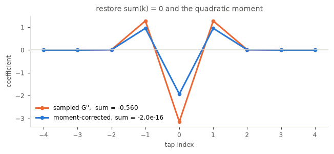

This is not a new idea. DIPlib does exactly this, and its author gave the recipe in the answer to the Stack Exchange question above — g2 -= np.mean(g2) then g2 /= np.sum(g2 * x**2) / 2.0. VIGRA does the same in initGaussianDerivative. ITK avoids the problem from the other side, building Lindeberg’s discrete analogue and convolving with a difference operator, which sums to zero by construction. Only SciPy samples and leaves it, and only scikit-image works around SciPy rather than correcting the kernel.

Against the standard¶

rows = []
for sigma in (0.4, 0.5, 1.0, 1.5, 3.0):
    tw, ti = border_and_interior(two_pass, PHOTO, sigma)
    ow, oi = border_and_interior(one_pass, PHOTO, sigma)
    rows.append({
        "sigma": sigma,
        "two-pass, worst": f"{tw:.1%}",
        "two-pass, interior": f"{ti:.1%}",
        "one-pass, worst": f"{ow:.1%}",
        "one-pass, interior": f"{oi:.1%}",
    })
show_table(pd.DataFrame(rows))

From sigma = 1.5 upwards the one-pass column is zero in both places: the border band of about a fifth of the peak becomes floating-point noise, and the interior stays exact. At sigma = 1 the worst error falls from 19% to 1.8%, and the interior error — the lost gain of section 5 — falls with it.

Below sigma = 1 the one-pass scheme is far better than the two-pass one, 18% against 98%, and is not good. Its remaining error is no longer at the border: the worst and interior figures are now the same number, so what is left is the aliasing residual, spread across the image. Correcting the moments does not remove that, and the last part of this section says why.

sigma = 1.5
truth = gold_hessian(PHOTO, sigma)
gap_two = np.abs(two_pass(PHOTO, sigma)[1] - truth[1])
gap_one = np.abs(one_pass(PHOTO, sigma)[1] - truth[1])

rows, cols = np.indices(PHOTO.shape)
to_edge = np.minimum(np.minimum(rows, cols),
                     np.minimum(PHOTO.shape[0] - 1 - rows,
                                PHOTO.shape[1] - 1 - cols))

fig, axes = plt.subplots(1, 2, figsize=(8.4, 3.0),
                         gridspec_kw={"width_ratios": [1, 1.4]})
image = show(axes[0], truth[1], "the standard, mixed element", diverging=True)
fig.colorbar(image, ax=axes[0], fraction=0.046)

for gap, name, colour in ((gap_two, "two-pass", C_TWO), (gap_one, "one-pass", C_ONE)):
    profile = [gap[to_edge == d].max() for d in range(25)]
    axes[1].semilogy(range(25), profile, color=colour, lw=2, label=name)
axes[1].set_xlabel("distance from the border, pixels", fontsize=8, color=MUTED)
axes[1].set_ylabel("worst error at that depth", fontsize=8, color=MUTED)
recede(axes[1], "where the error lives")
axes[1].legend(frameon=False, fontsize=8)
fig.suptitle(f"error against the standard, mixed element, sigma = {sigma}", y=1.03)
fig.tight_layout()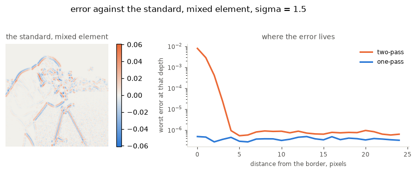

The profile is the whole of it. The two-pass error starts four orders of magnitude above the one-pass error at the outermost pixel and falls to meet it about five pixels in; from there the two curves lie together. So the two-pass scheme is not worse everywhere, it is worse in a band — and the band is where the second call’s invented boundary values reach.

The floor both curves settle on, around 5e-7, is not zero. It is this notebook’s standard disagreeing with both methods by the residual of its own construction, which is the honest limit of what can be claimed here: below that level, the reference cannot referee.

The order inconsistency goes with it, not by being reduced but by ceasing to exist: [2, 0] and [0, 2] are each other’s mirror and [1, 1] is its own, so relabelling the axes permutes the three results and changes nothing else.

def one_pass_xy(image, sigma):
    return one_pass(image, sigma)[::-1]


scale = max(np.abs(e).max() for e in one_pass(PHOTO, 1.5))
gap = max(np.abs(a - b).max()
          for a, b in zip(one_pass(PHOTO, 1.5), one_pass_xy(PHOTO, 1.5)[::-1])) / scale
print(f"one-pass, order='rc' against order='xy': {gap:.1e} of the peak")

one-pass, order='rc' against order='xy': 0.0e+00 of the peak

And truncate = 100 can go, which is what pays for the change.

import time


def best_of(f, n=5):
    f()
    return min([(lambda t0: (f(), time.perf_counter() - t0)[1])(time.perf_counter())
                for _ in range(n)])


rows = []
for sigma in (0.5, 1.0, 1.5, 3.0):
    t_two = best_of(lambda: two_pass(PHOTO, sigma))
    t_one = best_of(lambda: one_pass(PHOTO, sigma))
    rows.append({
        "sigma": sigma,
        "two-pass (ms)": t_two * 1e3,
        "one-pass (ms)": t_one * 1e3,
        "ratio": t_one / t_two,
    })
show_table(pd.DataFrame(rows), floatfmt=".2f")

Faster as well as more accurate, and dramatically so below sigma = 1, because the guard that made the kernel a hundred taps wide is no longer needed.

What this does not fix. Correcting the moments does not undo the aliasing. Sampling folds everything above the Nyquist frequency back into the band, and no choice of coefficients unfolds it. What the two conditions do is pin the operator to the ideal at zero frequency, which removes the two errors that are wrong for every image — a response to constants, and the wrong gain on smooth features. A residual remains at high frequency and grows toward Nyquist. It matters least where the method is used, because smoothing at scale sigma is precisely what removes the content the residual would affect.

# Gain on a pure sinusoid row: moment repair fixes DC, not the approach to Nyquist.
def sine_gain(method, sigma, waves):
    """Peak response / exact (−ω² e^{−σ²ω²/2}) for f = cos(ω j), ω = 2π / waves."""
    width = 512
    j = np.arange(width, dtype=float)
    gains = []
    for period in waves:
        omega = 2 * np.pi / period
        row = np.cos(omega * j)
        image = np.repeat(row[None, :], 64, axis=0)
        got = method(image, sigma)[2]          # Hjj: second deriv along columns
        # Exact continuous answer after Gaussian smoothing of scale sigma:
        # ∂²/∂x² (Gσ * cos(ωx)) = −ω² exp(−σ² ω² / 2) cos(ωx).
        exact_amp = (omega ** 2) * np.exp(-(sigma ** 2) * (omega ** 2) / 2)
        # Exclude a border margin so edge extension does not inflate the peak.
        gains.append(np.abs(got[32, 40:-40]).max() / exact_amp)
    return np.asarray(gains)


periods = np.array([4, 5, 6, 8, 10, 12, 16, 24, 32, 48, 64])
fig, ax = plt.subplots(figsize=(6.4, 2.8))
for method, name, colour in (
        (two_pass, "two-pass", C_TWO),
        (one_pass, "one-pass corrected", C_ONE),
):
    ax.plot(2 * np.pi / periods, sine_gain(method, 0.5, periods),
            color=colour, lw=2, marker="o", ms=4, label=name)
ax.axhline(1.0, color=INK, lw=1.2, label="exact")
ax.set_xlabel("spatial frequency ω, radians per pixel", fontsize=8, color=MUTED)
ax.set_ylabel("gain / exact", fontsize=8, color=MUTED)
recede(ax, "sigma = 0.5: DC is repaired, the Nyquist end is not")
ax.legend(frameon=False, fontsize=8)
fig.tight_layout()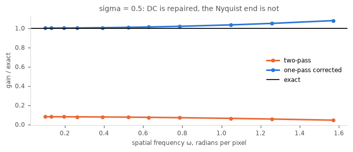

8. What `mode` does, and to which method¶

mode says how to continue the image past its edge. It is a statement about what is outside, so it cannot touch the interior: any method whose interior moves when mode changes has a defect that has nothing to do with boundaries. That makes it a useful probe, and the three methods answer it differently.

The standard has to be computed in the matching mode, or the comparison measures the mismatch. This is the section the DCT cannot referee: its boundary rule is half-sample reflection by construction, so four of these five are out of its reach and the supersampler does the work.

The check below is refinement stability, which section 3.6 showed is a partial test — it sees the fine-grid kernels and not the reconstruction. It is reported here for what it is; what makes the reference sound at the border is the periodic padding of section 3.2, and the agreement with the DCT at reflect.

MODES = ("nearest", "reflect", "mirror", "wrap", "constant")

rows = []
for mode in MODES:
    coarse = gold_hessian(PHOTO, 1.5, factor=2, mode=mode)
    finer = gold_hessian(PHOTO, 1.5, factor=4, mode=mode)
    scale = max(np.abs(e).max() for e in finer)
    gap = max(np.abs(a - b).max() for a, b in zip(coarse, finer)) / scale
    row = {"mode": mode, "k=2 vs k=4": f"{gap:.1e}"}
    if mode == "reflect":          # the one mode the exact standard can check
        row["vs dct"] = f"{error_against(finer, dct_hessian(PHOTO, 1.5), slice(None)):.1e}"
    rows.append(row)
show_table(pd.DataFrame(rows).fillna("—"))

def mode_error(method, sigma, mode, margin=20):
    truth = gold_hessian(PHOTO, sigma, mode=mode)
    got = method(PHOTO, sigma, mode=mode)
    scale = max(np.abs(e).max() for e in truth)
    inner = (slice(margin, -margin),) * 2
    return (max(np.abs(a - b).max() for a, b in zip(got, truth)) / scale,
            max(np.abs(a[inner] - b[inner]).max() for a, b in zip(got, truth)) / scale)


print("sigma = 1.5, worst error anywhere / interior only")
rows = []
for mode in MODES:
    row = {"mode": mode}
    for label, method in (("route A", route_a), ("two-pass", two_pass),
                          ("one-pass", one_pass)):
        whole, inner = mode_error(method, 1.5, mode)
        row[f"{label}, worst"] = f"{whole:.1%}"
        row[f"{label}, interior"] = f"{inner:.1%}"
    rows.append(row)
show_table(pd.DataFrame(rows))

sigma = 1.5, worst error anywhere / interior only

# Border error of the mixed element, two-pass, by mode — same diagnosis drawn.
sigma = 1.5
fig, axes = plt.subplots(1, 5, figsize=(12.0, 2.4))
for ax, mode in zip(axes, MODES):
    truth = gold_hessian(PHOTO, sigma, mode=mode)
    gap = np.abs(two_pass(PHOTO, sigma, mode=mode)[1] - truth[1])
    show(ax, gap, mode)
fig.suptitle("two-pass |error| against the standard, by mode (sigma = 1.5)",
             y=1.08)
fig.tight_layout()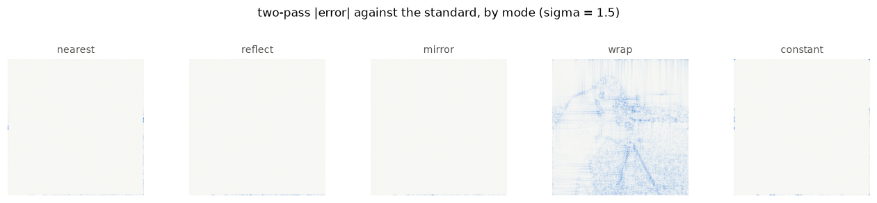

Route A ignores mode where it matters. Its interior error is 27.8% whatever mode says, which is right — mode should not reach the interior. But its border error changes with mode for a reason that is not to the caller’s credit: np.gradient applies one-sided differences at the first and last row and column, and no mode controls that. The smoothing honours the caller’s choice; the differencing then imposes an edge rule of its own on top.

# A quadratic separates the two stencils: the central difference is exact on
# it, a one-sided difference is not.
ramp = np.arange(7.0) ** 2
show_table(pd.DataFrame({
    "x": np.arange(7),
    "exact 2x": 2 * np.arange(7.0),
    "np.gradient": np.gradient(ramp),
}))
print("interior uses (f[n+1] - f[n-1]) / 2 and is exact here;")
print("the two ends fall back to a one-sided difference and are not.")
print("No value of `mode` reaches that choice — it is made inside np.gradient.")

interior uses (f[n+1] - f[n-1]) / 2 and is exact here;
the two ends fall back to a one-sided difference and are not.
No value of `mode` reaches that choice — it is made inside np.gradient.

nearest and wrap come off best for route A, at 27.8% — no worse at the border than in the interior — because an edge-replicated or wrapped image is locally smooth across the seam, so a one-sided difference happens to be close. reflect and mirror are worst, at 43.6% and 41.4%: reflection makes the true derivative zero at the edge by symmetry, and a one-sided estimate does not know that.

That 27.8% interior figure is worth a note of its own, because section 4 put route A at about 5% on a smooth Gaussian (SOLO). Both are right. The floor is sin(w)**2 / w**2, which depends on what frequencies the image contains, and a photograph contains far more high-frequency content than a single Gaussian blob.

rows = []
for name, image, region in (
    ("solo Gaussian", solo, SCENE_INTERIOR),
    ("camera", PHOTO, slice(35, -35)),
):
    truth = gold_hessian(image, 1.5, mode="nearest")
    got = route_a(image, 1.5, mode="nearest")
    scale = max(np.abs(e).max() for e in truth)
    err = max(np.abs(a[region, region] - b[region, region]).max()
              for a, b in zip(got, truth)) / scale
    rows.append({"image": name, "route A, interior": f"{err:.1%}"})
show_table(pd.DataFrame(rows))

The two-pass scheme is exact under wrap, and only under wrap. Its interior is exact in every mode, as it should be. Its border error runs from about 19% to 60% — and falls to the interior floor (a few parts in ten thousand, printing as zero at one decimal) for periodic boundaries.

That is the diagnosis of section 6 confirmed from the other side. The scheme fails because the second call re-extends an array the first has already smoothed, and the rule it applies is the rule for an image, not for a derivative field. Under wrap there is no such thing as outside: a periodic signal’s continuation is exact, it is the same for the image and for every field derived from it, and applying it twice is applying it once. Remove the guesswork and the border defect goes with it.

The ranking of the other four follows the same logic. nearest is the least bad at 18.9%, because a replicated edge is at least a plausible continuation of a smoothed field. reflect, mirror and constant are all worse, at 45%, 61% and 59%, because each asserts something specific about the derivative field outside that is not true of it.

The one-pass scheme does not care. Zero in every mode, because each axis is extended once and a boundary extension along one axis commutes exactly with filtering along another. There is no second extension to be wrong.

What to take from it¶

Do not choose a mode to dodge this. wrap makes the two-pass border error vanish into the interior floor, and almost no image is periodic: choosing it would replace a border artefact with a different and larger one, of the left edge bleeding into the right. The right reading is diagnostic — the fact that one mode removes the border error entirely is the strongest evidence that the defect is the extension and not the arithmetic.

For a caller today, mode='nearest' is the least damaging choice with the shipped scheme, at a third of the error of mirror. That is a workaround, and it costs nothing to say so. After the one-pass change the choice goes back to being what the documentation says it is: a statement about what lies outside the image, with no effect on the answer inside it.

9. What changes for the callers¶

hessian_matrix is not used directly by most of the people who depend on it. It is consumed by four ridge filters, and the question that decides whether this is worth doing is what happens to them.

The same standard applies. A ridge filter run on a once-extended image and cropped back is the answer it should give: the interior pixels have seen no edge, so nothing in the result is a border artefact. Comparing each filter against that says how much of its output is real.

import importlib
import sys
from unittest import mock

PAD = 110                                   # clears truncate = 100 at sigma = 1
RIDGE = dict(mode="nearest")                # matches np.pad(..., mode='edge')
padded_photo = np.pad(PHOTO, PAD, mode="edge")
FILTERS = [("frangi", frangi), ("sato", sato),
           ("meijering", meijering), ("hessian", hessian)]

package = sys.modules[frangi.__module__].__package__.rsplit(".", 1)[0]
corner_mod = importlib.import_module(f"{package}.feature.corner")


def as_hessian_matrix(rule):
    """Wrap a Hessian rule in the `hessian_matrix` signature, ready to patch in."""
    def replacement(image, sigma=1, mode="reflect", cval=0, order="rc",
                    use_gaussian_derivatives=True):
        return rule(ski.util.img_as_float(image), sigma, mode=mode)
    return replacement


def ridge_border_frame():
    rows = []
    for name, f in FILTERS:
        direct = f(PHOTO, **RIDGE)
        reference = f(padded_photo, **RIDGE)[PAD:-PAD, PAD:-PAD]
        gap = np.abs(direct - reference)
        rows.append({
            "filter": name,
            "worst vs pad-once": f"{gap.max() / max(np.abs(reference).max(), 1e-12):.1%}",
            "30 px in": f"{gap[30:-30, 30:-30].max():.1e}",
        })
    return pd.DataFrame(rows)


display(Markdown("**as shipped, two-pass**"))
show_table(ridge_border_frame().set_index("filter"))
with mock.patch.object(corner_mod, "hessian_matrix", as_hessian_matrix(one_pass)):
    display(Markdown("**with one-pass corrected kernels**"))
    show_table(ridge_border_frame().set_index("filter"))

Three of the four become exact — not improved, exact. meijering does not, and the residue is its interior figure, unchanged: it divides each scale by that scale’s maximum over the whole image, so its output at a pixel depends on pixels arbitrarily far away, and a once-extended image is a larger image with a different maximum. That is a separate defect, in meijering alone, which the border fix exposes rather than causes. on_meijering.md is about it.

sigma_sweep = dict(sigmas=(1, 3, 5), mode="nearest")
before = frangi(PHOTO, **sigma_sweep)
with mock.patch.object(corner_mod, "hessian_matrix", as_hessian_matrix(one_pass)):
    after = frangi(PHOTO, **sigma_sweep)

fig, axes = plt.subplots(1, 3, figsize=(9.6, 3.0))
show(axes[0], before, "frangi, as shipped")
show(axes[1], after, "frangi, one-pass corrected")
image = show(axes[2], np.abs(before - after), "what changes")
fig.colorbar(image, ax=axes[2], fraction=0.046)
fig.suptitle("the change is a border band, and the smallest scale", y=1.03)
fig.tight_layout()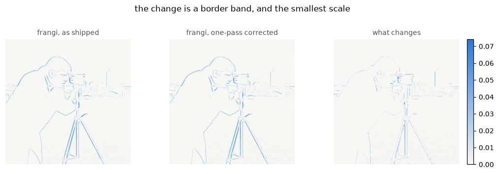

Why the new numbers are the better ones¶

Output changes, so the question is not “are they different” but “is the difference an improvement”. Three things answer it, and none of them is a preference.

At the border, the old values are wrong against a standard fixed in advance. Not different from the new ones — wrong, by about a fifth of the peak response, against a reference that applies the documented boundary rule once and is agreed before either method is run.

In the interior below sigma = 1, the old values lose gain. Section 5 measured the two-pass scheme reporting 8% of the curvature of a quadratic at sigma = 0.5. The corrected kernel reports it exactly. A filter sweeping small scales was reading real structure as nearly flat.

The order argument stops meaning two things. Today order='rc' and order='xy' differ by 11% on this photograph, and by 40% on less forgiving data, for a quantity documented as one tensor in two labellings. After the change they are the same numbers permuted, which is what the docstring already claims.

show_table(pd.DataFrame([
    {"check": "border error, sigma >= 1.5",
     "two-pass": "~19% of the peak", "one-pass corrected": "floating-point noise"},
    {"check": "interior, sigma >= 1.5",
     "two-pass": "exact", "one-pass corrected": "exact"},
    {"check": "quadratic gain at sigma = 0.5",
     "two-pass": "0.08", "one-pass corrected": "1.00"},
    {"check": "response to a constant",
     "two-pass": "0", "one-pass corrected": "~1e-17"},
    {"check": "order='rc' vs 'xy'",
     "two-pass": "~11% apart", "one-pass corrected": "identical"},
    {"check": "cost at sigma = 1",
     "two-pass": "1x", "one-pass corrected": "about 0.05x"},
]))

The one place the old scheme is better is a test it was designed against: on a perfectly constant image it returns exactly zero, where the corrected kernel returns 1e-17. That is the difference between a symmetry and a numerical correction, and it is not a reason to prefer it.

What is still open¶

The corrected kernel is not the last word. It fixes the operator at zero frequency and leaves a residual that grows toward Nyquist, so at sigma well below 1 no kernel repair rescues the method — only a larger scale, a finer grid, or a different family of method.

That third option is the one the cited paper argues for, and this notebook has been using it as a yardstick without putting it on trial. Rey-Otero and Delbracio conclude that “the only method that allows to compute accurately the Gaussian scale-space is the Fourier based convolution”, and that sampled Gaussians are sound only above sigma about 0.8 — which is section 7’s residual, reached independently and four years earlier. dct_hessian is not merely a standard: it is a candidate implementation, and on the evidence here it is the accurate one at every scale.

It is not proposed as the implementation, for reasons this notebook has not measured. It is global rather than separable and local, so cost scales as N log N over the whole image rather than with the kernel, and it cannot offer mode: the boundary rule is half-sample reflection by construction, where callers currently choose among five. Whether a spectral path should exist alongside the kernel one, for the small-sigma regime where kernels cannot be repaired, is a real question and is left open here rather than answered. hessian_matrix_det(approximate=True) and blob_doh route through box filters over integral images and are untouched by any of this; they have their own border defect, larger than this one, described in on_blob_dog.md. And meijering’s normalisation needs deciding on its own terms.

Measured with scikit-image from this working tree, on the 201×201 Gaussian scenes (SOLO and multi-blob/ridge SCENE, closed form) and the 256×256 camera photograph, against the IPOL DCT continuous Hessian and a supersampled reference at refinement factor 4.

print(f"scikit-image {ski.__version__}")
print(f"scipy        {__import__('scipy').__version__}")

scikit-image 0.26.1rc0.dev0
scipy        1.18.1