skimage.feature.structure_tensor and skimage.feature.hessian_matrix both
take an order parameter, documented as choosing between two labellings of the
same tensor. For one of them that is true. For the other it is not, and
following the difference leads to a border defect that reaches a third of the
signal and shows up in frangi, sato, meijering and hessian.
This notebook explains what each function computes, why they differ, what the correct answer is, and what a fix changes.
The border discrepancy is a finite-array implementation issue. The scale-space papers define convolution on an infinite grid; the reference used here is the explicit once-extended finite-array construction chosen by this notebook.
Coordinates are in array order throughout: the first index runs down the picture, the second runs right.
import warnings

import numpy as np
import scipy.ndimage as ndi
import matplotlib.pyplot as plt
from matplotlib.colors import LinearSegmentedColormap, TwoSlopeNorm

warnings.simplefilter("ignore")  # the use_gaussian_derivatives FutureWarning
import skimage as ski
from skimage.feature import structure_tensor, hessian_matrix
from skimage.filters import frangi, sato, meijering, hessianfatal: not a git repository (or any of the parent directories): .git
fatal: not a git repository (or any of the parent directories): .git
# Comparator.
import cv2
# Slots 1 to 3 of the reference categorical palette, validated all-pairs.
C_ONE = "#2a78d6"
C_TWO = "#eb6834"
C_THREE = "#1baf7a"
INK, MUTED, GRID = "#0b0b0b", "#52514e", "#dedcd5"
# Sequential: one hue, light to dark. Diverging: two hues, neutral midpoint.
SEQ = LinearSegmentedColormap.from_list("seq", ["#f7f7f4", C_ONE])
DIV = LinearSegmentedColormap.from_list("div", [C_ONE, "#f2f1ec", C_TWO])
plt.rcParams.update(
{"figure.dpi": 110, "font.size": 9, "axes.titlesize": 9,
"axes.titlecolor": MUTED, "figure.facecolor": "white"}
)
def show(ax, data, title=None, cmap=SEQ, diverging=False, vmax=None):
"""Draw an array with recessive axes; diverging data is centred on zero."""
if diverging:
m = vmax if vmax is not None else np.abs(data).max() or 1.0
im = ax.imshow(data, cmap=DIV, norm=TwoSlopeNorm(0, -m, m))
else:
im = ax.imshow(data, cmap=cmap, vmin=0, vmax=vmax)
ax.set_xticks([])
ax.set_yticks([])
for spine in ax.spines.values():
spine.set_visible(False)
if title is not None:
ax.set_title(title)
return im
rng = np.random.default_rng(7)
IMG = rng.random((60, 70)) # asymmetric and non-square, so axis order shows
SIGMA, MODE = 1.5, "nearest"1. What a Hessian is, and why an image needs a scale
The Hessian matrix collects the second partial derivatives of a function. For a 2-D image it has three distinct entries, because mixed partials are equal:
    H = | Hrr  Hrc |
        | Hrc  Hcc |
Its eigenvalues describe the local curvature. Two large negative eigenvalues
mark a bright blob; one large and one near zero mark a ridge. That is the basis
of ridge detection, which is
what frangi, sato and meijering do, and of the determinant-of-Hessian
blob detector.
An image is a grid of samples, not a differentiable function, and differencing
neighbouring pixels amplifies noise without limit. The standard remedy is to
fix a scale: convolve with a Gaussian of width sigma, and differentiate
that instead. This is the basis of
scale space. So the Hessian of an
image is always the Hessian at a scale, and sigma is part of the
definition rather than a tuning knob.
# A Gaussian blob, and the three distinct entries of its Hessian.
BLOB_N, BLOB_S = 121, 4.0
centre = BLOB_N // 2
bi, bj = np.indices((BLOB_N, BLOB_N), dtype=float)
radius2 = (bi - centre) ** 2 + (bj - centre) ** 2
blob = np.exp(-radius2 / (2 * BLOB_S**2)) / (2 * np.pi * BLOB_S**2)

entries = hessian_matrix(blob, sigma=2.0, mode="nearest",
                         use_gaussian_derivatives=True)

fig, axes = plt.subplots(1, 4, figsize=(10.0, 2.6))
show(axes[0], blob[30:-30, 30:-30], "the blob")
for ax, name, entry in zip(axes[1:], ("Hrr", "Hrc", "Hcc"), entries):
    show(ax, entry[30:-30, 30:-30], name, diverging=True)
fig.suptitle("a blob and its second derivatives at sigma = 2", y=1.04)
fig.tight_layout()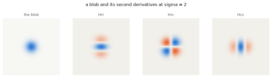
Hrr is negative in a band across the middle, where the blob curves downwards
along the row axis, and positive in the two lobes above and below it where that
curvature reverses. Hcc is the same pattern turned through a right angle,
because it differentiates along the other axis. Hrc is the saddle term: four
lobes of alternating sign, vanishing along both axes.
2. The two ways hessian_matrix computes it
Convolution and differentiation commute, so for a Gaussian G and an image
f:
d/dx (G * f) == (dG/dx) * fEither side is a valid route to a smoothed derivative, and
use_gaussian_derivatives chooses between them.
use_gaussian_derivatives=False takes the left-hand side. It smooths with
gaussian, then calls np.gradient twice. The derivative is an ordinary
finite difference, taken on the blurred image.
use_gaussian_derivatives=True takes the right-hand side. It convolves
with derivatives of the Gaussian directly, through the order argument of
scipy.ndimage.gaussian_filter.
It applies two successive first-order passes rather than one second-order
pass, and each pass uses sigma / sqrt(2). For continuous Gaussians, two
Gaussians of that width compose to a Gaussian of width sigma. SciPy uses
sampled and truncated kernels, so this is the continuous target, not an exact
discrete identity; Lindeberg (1993)
and Lindeberg (2024)
describe the loss of the semigroup property for sampled Gaussians, especially
at fine scales.
single = ndi.gaussian_filter(blob, 2.0, mode="nearest")
halved = ndi.gaussian_filter(
    ndi.gaussian_filter(blob, 2.0 / np.sqrt(2), mode="nearest"),
    2.0 / np.sqrt(2), mode="nearest",
)
print(f"one pass at sigma vs two at sigma/sqrt(2): "
      f"max difference {np.abs(single - halved).max():.2e}")
one pass at sigma vs two at sigma/sqrt(2): max difference 1.92e-07
That continuous composition is why the two-pass scheme is used. The measured difference above is specific to this image, boundary mode, and scale. The two separate boundary extensions are also where the border problem in section 7 comes from.
3. Which of the two is more accurate
The choice is not arbitrary, and it can be measured against a known answer. A
Gaussian blob has an analytic Hessian, and a Gaussian smoothed by a Gaussian is
another Gaussian with t**2 = s**2 + sigma**2. So the smoothed Hessian is
analytic too.
def analytic_hessian(sigma):
    """The exact Hessian of the blob after smoothing at `sigma`."""
    t2 = BLOB_S**2 + sigma**2
    g = np.exp(-radius2 / (2 * t2)) / (2 * np.pi * t2)
    di, dj = bi - centre, bj - centre
    return [g * (di**2 / t2**2 - 1 / t2),
            g * (di * dj / t2**2),
            g * (dj**2 / t2**2 - 1 / t2)]


INTERIOR = slice(30, -30)


def relative_error(computed, sigma):
    """Worst error over the three entries, away from the border."""
    truth = analytic_hessian(sigma)
    scale = max(np.abs(e).max() for e in truth)
    return max(np.abs(c[INTERIOR, INTERIOR] - e[INTERIOR, INTERIOR]).max()
               for c, e in zip(computed, truth)) / scale
sigmas = [0.6, 0.8, 0.9, 1.0, 1.5, 2.0, 3.0, 5.0]
finite, gaussian_deriv = [], []
for sigma in sigmas:
finite.append(relative_error(
hessian_matrix(blob, sigma=sigma, mode="nearest",
use_gaussian_derivatives=False), sigma))
gaussian_deriv.append(relative_error(
hessian_matrix(blob, sigma=sigma, mode="nearest",
use_gaussian_derivatives=True), sigma))
print(f"{'sigma':>6}{'finite differences':>21}{'gaussian derivatives':>23}")
for sigma, a, b in zip(sigmas, finite, gaussian_deriv):
print(f"{sigma:>6}{a:>20.2%}{b:>23.2%}") sigma finite differences gaussian derivatives
0.6 5.77% 63.08%
0.8 5.77% 9.64%
0.9 5.72% 2.48%
1.0 5.66% 0.52%
1.5 5.28% 0.00%
2.0 4.83% 0.00%
3.0 3.89% 0.00%
5.0 2.39% 0.00%
For this blob, interior crop, and list of tested scales, the Gaussian-derivative
route reaches floating-point agreement above sigma = 1, while finite
differences stay wrong by a few percent. This is a measurement of this test,
not a general exactness claim. Lindeberg’s 2024 discretization
study reports
that sampled Gaussian derivatives are usually accurate above about one pixel,
but that the threshold depends on derivative order and task. Below about
sigma = 0.85 they swap places here, and the Gaussian route degrades sharply:
its kernels are then narrower than a pixel and badly sampled. That is the
aliasing the docstring warns about when it advises against a sigma much
less than 1. The next subsection says what that word means here, what the
source’s truncate = 100 line does about it, and why that choice forces enormous
image padding later.
Two further points are revisited with the fixes. The aliasing itself is not
repairable — it is lost information — but its two unconditional consequences
are, which is Fix C and the subject of the last part of this section; and the
crossover itself moves with the test image, because blob is very smooth and
that flatters finite differences more than a textured image would.
Aliasing, truncate = 100, and padding
SciPy builds each Gaussian-derivative FIR by sampling the continuous formula
on the integer grid, normalizing the sampled zeroth-order Gaussian first, and
truncating at radius
L = int(truncate * sigma + 0.5). Call each coefficient a tap (standard FIR
jargon; see
Wikipedia: Finite impulse response).
For a second derivative this is therefore the normalized-sampled-derivative
variant of the continuous shape
g(x) * (x**2 - sigma**2) / sigma**4 with g a normalised Gaussian.
def gaussian_taps(sigma, order, trunc):
    """The 1-D kernel `gaussian_filter` builds, from the explicit formula."""
    lw = int(trunc * sigma + 0.5)
    x = np.arange(-lw, lw + 1).astype(float)
    g = np.exp(-(x**2) / (2 * sigma**2))
    g /= g.sum()
    if order == 0:
        return x, g
    if order == 1:
        return x, g * (x / sigma**2)
    return x, g * ((x**2 - sigma**2) / sigma**4)
A faithful discrete second derivative must annihilate constants and reproduce
quadratics: sum(k) == 0 and sum(k * x**2) / 2 == 1. Sampling breaks both
once sigma drops below about one pixel, and widening the support does not
repair them.
print("order=2 moments; want sum = 0 and sum k*x**2/2 = 1")
print(f"{'sigma':>7}{'truncate':>10}{'n taps':>8}{'sum':>12}{'sum k*x**2/2':>14}")
for sigma in (0.5, 0.7, 1.0):
    for trunc in (8, 100):
        x, k = gaussian_taps(sigma, 2, trunc)
        print(f"{sigma:>7}{trunc:>10}{k.size:>8}"
              f"{k.sum():>12.2e}{(k * x**2).sum() / 2:>14.4f}")
order=2 moments; want sum = 0 and sum k*x**2/2 = 1
sigma truncate n taps sum sum k*x**2/2
0.5 8 9 -5.60e-01 1.3408
0.5 100 101 -5.60e-01 1.3408
0.7 8 13 -4.97e-03 1.0175
0.7 100 141 -4.97e-03 1.0175
1.0 8 17 -2.11e-07 1.0000
1.0 100 201 -2.11e-07 1.0000
Why call that aliasing. The continuous second derivative of a Gaussian has
Fourier transform proportional to -ω² exp(-σ² ω² / 2). Small sigma spreads
that spectrum past the Nyquist frequency π (one cycle per two pixels).
Sampling on the integers folds the out-of-band energy back into
[-π, π], so the discrete taps are not the continuous operator restricted to
the grid. The Gaussian is not band-limited; higher derivative order widens the
spectrum further, which is why a first-derivative kernel survives sampling
better than a second-derivative one (an odd kernel still sums to zero by
symmetry; an even one need not).
The visible symptoms are exactly the failed moments: a non-zero sum is a
DC leak (flat brightness reads as curvature), and a wrong second moment is
gain error. Those are properties of the few central taps. At
sigma = 0.5 essentially all the mass sits in x ∈ {-1, 0, 1} whether
truncate is 8 or 100 — the table above is the measurement.
What truncate = 100 is, and what it was for. The source sets it in
feature/corner.py, with a comment that gives the reasoning in full:
    # For small sigma, the SciPy Gaussian filter suffers from aliasing and edge
    # artifacts, given that the filter will approximate a sinc or sinc
    # derivative which only goes to 0 very slowly (order 1/n**2). Thus, we use
    # a much larger truncate value to reduce any edge artifacts.
    truncate = 8 if all(s > 1 for s in sigma) else 100
The diagnosis in the first clause is right: at small sigma there is aliasing.
The remedy follows from the second clause, and that is where it goes wrong. The
argument is that the kernel decays like a sinc, as 1/n**2, so a window of
ordinary width would chop off tails that still carry weight — hence a window
twelve times wider.
A sampled Gaussian derivative does not decay like a sinc. It decays like a Gaussian.
x_far, k_far = gaussian_taps(0.5, 2, 100)
peak = np.abs(k_far).max()
centre = k_far.size // 2

print("sigma = 0.5, truncate = 100: how fast do the taps really fall off?")
print(f"{'n':>4}{'|k[n]| / peak':>16}{'1/n**2, as the comment assumes':>33}")
for n in (1, 2, 3, 4, 8):
    print(f"{n:>4}{abs(k_far[centre + n]) / peak:>16.2e}{1.0 / n**2:>33.2e}")

beyond = np.abs(k_far[np.abs(x_far) > 4]).sum() / np.abs(k_far).sum()
print(f"\nof {k_far.size} taps, those beyond |n| > 4 hold {beyond:.1e} of the "
      f"total absolute weight")
sigma = 0.5, truncate = 100: how fast do the taps really fall off?
n |k[n]| / peak 1/n**2, as the comment assumes
1 4.06e-01 1.00e+00
2 5.03e-03 2.50e-01
3 5.33e-07 1.11e-01
4 7.98e-13 6.25e-02
8 6.56e-54 1.56e-02
of 101 taps, those beyond |n| > 4 hold 2.1e-20 of the total absolute weight
At n = 8 the real coefficient is fifty-two orders of magnitude below what a
1/n**2 tail would be. The 92 extra taps that truncate = 100 buys at
sigma = 0.5 carry 2e-20 of the kernel’s weight between them. They are not
small-but-helpful; they are zero.
So the guard cannot work, and measurement confirms it does not — neither on the moments nor on the filtered output:
noise = np.random.default_rng(7).random((60, 70))

print("same filter, two truncate values")
print(f"{'sigma':>7}{'d(sum)':>12}{'d(second moment)':>20}"
      f"{'max |output difference|':>26}")
for sigma in (0.5, 0.7, 1.0, 1.5):
    x8, k8 = gaussian_taps(sigma, 2, 8)
    x100, k100 = gaussian_taps(sigma, 2, 100)
    d_sum = abs(k8.sum() - k100.sum())
    d_m2 = abs((k8 * x8**2).sum() - (k100 * x100**2).sum())
    narrow = ndi.gaussian_filter(noise, sigma, order=[2, 0], mode="nearest",
                                 truncate=8)
    wide = ndi.gaussian_filter(noise, sigma, order=[2, 0], mode="nearest",
                               truncate=100)
    print(f"{sigma:>7}{d_sum:>12.1e}{d_m2:>20.1e}"
          f"{np.abs(narrow - wide).max():>26.1e}")
same filter, two truncate values
sigma d(sum) d(second moment) max |output difference|
0.5 0.0e+00 0.0e+00 0.0e+00
0.7 4.3e-17 4.4e-16 0.0e+00
1.0 9.6e-17 1.3e-14 1.4e-16
1.5 8.2e-16 1.4e-13 6.9e-16
Where the guard is active and the aliasing is real — sigma of 0.5 and 0.7 —
the two kernels are bit-identical and so is the output. Above that the widest
disagreement anywhere is 7e-16, floating-point noise. truncate = 100 is not
a weak remedy for the aliasing, it is not a remedy at all: the problem is in the
few central taps, and no width of window fixes a tap that is already present and
wrong.
What it does do is cost. That is the rest of this subsection.
fig, axes = plt.subplots(1, 2, figsize=(9.0, 2.8), sharey=True)
for ax, trunc in zip(axes, (8, 100)):
    x, k = gaussian_taps(0.5, 2, trunc)
    ax.axhline(0, color=GRID, lw=0.8)
    ax.vlines(x, 0, k, color=C_ONE, lw=1.0)
    ax.plot(x, k, "o", color=C_ONE, ms=3)
    ax.set_xlim(-8 if trunc == 8 else -20, 8 if trunc == 8 else 20)
    ax.set_title(f"sigma = 0.5, truncate = {trunc}  "
                 f"({k.size} taps, sum = {k.sum():+.3f})")
    ax.set_xlabel("pixels from centre", fontsize=8, color=MUTED)
    ax.tick_params(labelsize=8, colors=MUTED)
    for s in ("top", "right"):
        ax.spines[s].set_visible(False)
fig.suptitle("same central taps; the extra width is nearly empty", y=1.04)
fig.tight_layout()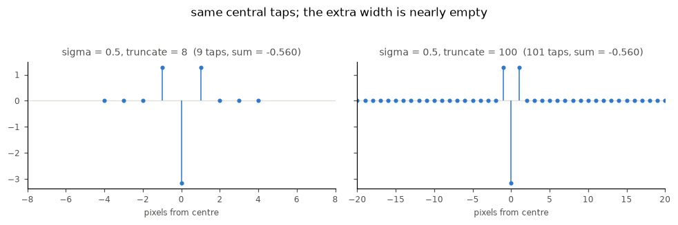
How that forces padding. Convolution support is set by the FIR radius
L = int(truncate * sigma + 0.5). Any pad-once reference, and Fix B later, must
clear that radius or the crop still feels the border, and the radius is twelve
times larger than it needs to be wherever the guard is active.
print(f"{'sigma':>7}{'guard active?':>15}{'radius used':>14}"
      f"{'radius without the guard':>27}")
for sigma in (0.5, 1.0, 1.01, 3.0, 5.0):
    active = not (sigma > 1)                     # the source's own test
    truncate = 100 if active else 8
    print(f"{sigma:>7}{('yes' if active else 'no'):>15}"
          f"{int(truncate * sigma + 0.5):>14}{int(8 * sigma + 0.5):>27}")
sigma guard active? radius used radius without the guard
0.5 yes 50 4
1.0 yes 100 8
1.01 no 8 8
3.0 no 24 24
5.0 no 40 40
At sigma = 1, where the guard is still on, it asks for a 100-pixel radius in
place of 8. That is the whole of the excess: a pad-once reference at that scale
needs a margin of about a hundred pixels rather than a dozen. The ridge-filter
comparison in section 9 pays it, and so does Fix B.
The guard is also why the numbers jump at sigma = 1.01: the test is
all(s > 1 for s in sigma), so a hair above one the radius falls from 100 to 8
and everything downstream gets cheaper at a stroke.
Treat truncate = 100 as a historical guard whose only measurable effect in
this notebook is cost. What to do instead is Fix C — which does not undo the
aliasing, because nothing can, but does remove the part of it that is wrong for
every image. Fix C’s subsection “what correcting the taps can and cannot do”
draws that line precisely.
How other libraries compute it
OpenCV has no Hessian function, but it has the parts: GaussianBlur for the
scale and Sobel for the derivatives. One catch is that cv2.Sobel returns
unnormalised kernels, so a direct comparison measures a scale factor rather
than an error. cv2.getDerivKernels shows the difference and supplies the
normalised form.
for dx, dy in ((2, 0), (1, 1)):
    raw = cv2.getDerivKernels(dx, dy, 3, normalize=False)
    normalised = cv2.getDerivKernels(dx, dy, 3, normalize=True)
    print(f"d{dx}{dy}  raw {raw[0].ravel()} x {raw[1].ravel()}"
          f"   normalised {normalised[0].ravel()} x {normalised[1].ravel()}")
d20 raw [ 1. -2. 1.] x [1. 2. 1.] normalised [ 1. -2. 1.] x [0.25 0.5 0.25]
d11 raw [-1. 0. 1.] x [-1. 0. 1.] normalised [-0.5 0. 0.5] x [-0.5 0. 0.5]
def opencv_hessian(image, sigma):
    """Blur at `sigma`, then take normalised Sobel second derivatives."""
    size = int(6 * sigma) | 1
    smoothed = cv2.GaussianBlur(image, (size, size), sigma,
                                borderType=cv2.BORDER_REPLICATE)
    out = []
    for dy, dx in ((2, 0), (1, 1), (0, 2)):
        kx, ky = cv2.getDerivKernels(dx, dy, 3, normalize=True)
        out.append(cv2.sepFilter2D(smoothed, cv2.CV_64F, kx, ky,
                                   borderType=cv2.BORDER_REPLICATE))
    return out


opencv = [relative_error(opencv_hessian(blob, s), s) for s in sigmas]
print(f"{'sigma':>6}{'finite':>10}{'gaussian':>11}{'opencv Sobel':>15}")
for sigma, a, b, d in zip(sigmas, finite, gaussian_deriv, opencv):
    print(f"{sigma:>6}{a:>9.2%}{b:>11.2%}{d:>15.2%}")
sigma finite gaussian opencv Sobel
0.6 5.77% 63.08% 106.64%
0.8 5.77% 9.64% 106.55%
0.9 5.72% 2.48% 106.52%
1.0 5.66% 0.52% 106.45%
1.5 5.28% 0.00% 106.29%
2.0 4.83% 0.00% 107.28%
3.0 3.89% 0.00% 107.51%
5.0 2.39% 0.00% 106.78%
fig, ax = plt.subplots(figsize=(6.2, 3.0))
for values, colour, label in ((finite, C_TWO, "finite differences"),
                              (gaussian_deriv, C_ONE, "gaussian derivatives"),
                              (opencv, C_THREE, "opencv Sobel")):
    # A log axis cannot show an exact zero, so the curve rests on a floor.
    ax.semilogy(sigmas, np.maximum(values, 1e-6), color=colour, linewidth=2,
                marker="o", markersize=4, label=label)
ax.set_xlabel("sigma", fontsize=8, color=MUTED)
ax.set_ylabel("worst relative error, floored at 1e-6", fontsize=8, color=MUTED)
ax.tick_params(labelsize=8, colors=MUTED)
for side in ("top", "right"):
    ax.spines[side].set_visible(False)
for side in ("left", "bottom"):
    ax.spines[side].set_color(GRID)
ax.legend(frameon=False, fontsize=8)
ax.set_title("accuracy against an analytic Hessian")
fig.tight_layout()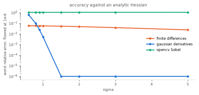
Pillow has no equivalent: ImageFilter offers fixed 3 by 3 kernels, with no
scale parameter and no second derivatives, so it does not enter this
comparison.
The ordering is stable: Gaussian derivatives above sigma = 1, then OpenCV’s
normalised Sobel, then our finite differences. This is the case for changing
the default, and it is separate from the border defect that the rest of this
notebook is about.
4. What order is supposed to mean
Both functions return the upper-diagonal elements of a symmetric 2x2 tensor.
With order='rc' they are named (Arr, Arc, Acc); with order='xy' they are
named (Axx, Axy, Ayy). Since x is the column axis and y the row axis,
Axx is Acc, Ayy is Arr, and Axy is Arc. So the documented contract
is that order reverses the list and changes nothing else.
The test suite says so too, in tests/skimage/feature/test_corner.py:
# verify results are equivalent, just reversed in order
assert_array_equal(Hxy, Hrc)
5. structure_tensor keeps that contract exactly
st_xy = structure_tensor(IMG, sigma=SIGMA, mode=MODE, order="xy")
st_rc = structure_tensor(IMG, sigma=SIGMA, mode=MODE, order="rc")
print("xy equals reversed rc, bit for bit:",
      all(np.array_equal(a, b) for a, b in zip(st_xy, st_rc[::-1])))
xy equals reversed rc, bit for bit: True
This is not luck. structure_tensor forms each element as a pointwise product
of two derivative images and then smooths it. The only element that could
differ is the mixed one, gaussian(d1 * d0) against gaussian(d0 * d1), and
IEEE multiplication is commutative — so gaussian receives bit-identical
input.
6. hessian_matrix does not
def hess(order, ugd):
    return hessian_matrix(IMG, sigma=SIGMA, mode=MODE, order=order,
                          use_gaussian_derivatives=ugd)

for ugd in (False, True):
    xy, rc = hess("xy", ugd), hess("rc", ugd)[::-1]
    worst = max(float(np.max(np.abs(a - b))) for a, b in zip(xy, rc))
    print(f"use_gaussian_derivatives={ugd!s:<5} "
          f"identical={all(np.array_equal(a, b) for a, b in zip(xy, rc))!s:<5} "
          f"max abs difference {worst:.3e}")
use_gaussian_derivatives=False identical=True max abs difference 0.000e+00
use_gaussian_derivatives=True identical=False max abs difference 4.022e-02
The np.gradient path agrees to rounding. The Gaussian-derivative path does
not — and that path is the one frangi, sato, meijering and hessian all
use, and the one the FutureWarning says will become the default.
xy = hess("xy", True)
rc = hess("rc", True)[::-1]

fig, axes = plt.subplots(1, 3, figsize=(9.0, 2.8))
show(axes[0], xy[1], "order='xy', mixed element", diverging=True)
show(axes[1], rc[1], "order='rc' reversed, mixed element", diverging=True)
im = show(axes[2], np.abs(xy[1] - rc[1]), "absolute difference")
fig.colorbar(im, ax=axes[2], fraction=0.046)
fig.suptitle("the same element, asked for two ways", y=1.02)
fig.tight_layout()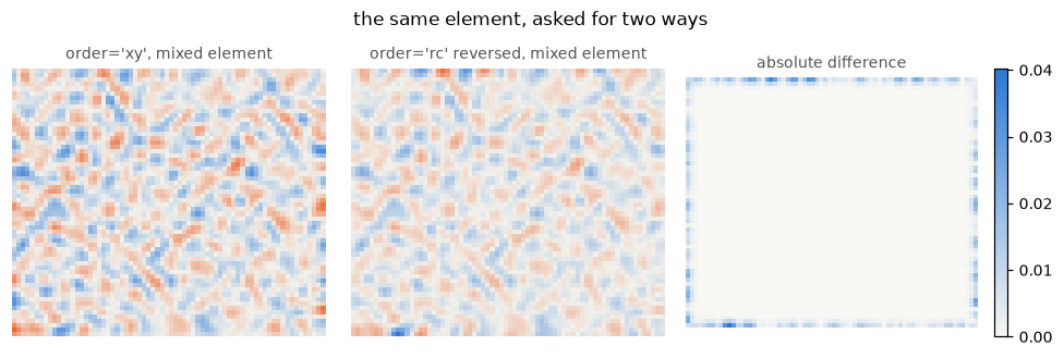
The difference is a ring around the border. Everything inside is identical.
7. Why: extensions commute across axes, not within one
mode says how to continue the image past its edge. Each call to
ndi.gaussian_filter applies that rule itself. The question is whether
composing calls preserves it.
P = 40
g1 = lambda a, ax: ndi.gaussian_filter1d(a, SIGMA, axis=ax, mode=MODE)

def error_vs_pad_once(f):
    return np.max(np.abs(f(IMG) - f(np.pad(IMG, P, mode="edge"))[P:-P, P:-P]))

print(f"{'composition':<48}{'error vs pad-once':>18}")
for label, f in [
    ("one pass on axis 0", lambda a: g1(a, 0)),
    ("axis 0, then axis 1   (different axes)", lambda a: g1(g1(a, 0), 1)),
    ("axis 0, axis 1, axis 0   (axis 0 twice)", lambda a: g1(g1(g1(a, 0), 1), 0)),
    ("axis 1, then axis 1   (same axis twice)", lambda a: g1(g1(a, 1), 1)),
]:
    print(f"{label:<48}{error_vs_pad_once(f):>18.2e}")
composition error vs pad-once
one pass on axis 0 0.00e+00
axis 0, then axis 1 (different axes) 0.00e+00
axis 0, axis 1, axis 0 (axis 0 twice) 3.46e-02
axis 1, then axis 1 (same axis twice) 7.82e-02
A boundary extension along one axis commutes exactly with filtering along a different axis, and not at all with filtering along the same axis.
Here is what the second call gets wrong. The first pass produces a derivative
field. Outside the image that field keeps varying for about a kernel radius
before it settles. mode='nearest' on the cropped field asserts instead that
it is constant from the edge onwards.
ss = SIGMA / np.sqrt(2)
kw0 = dict(mode=MODE, truncate=8)
row = 30

true_field = ndi.gaussian_filter(np.pad(IMG, P, mode="edge"), ss, order=[1, 0], **kw0)
have = ndi.gaussian_filter(IMG, ss, order=[1, 0], **kw0)

span = 24
outside = np.arange(-span, 0)
inside = np.arange(0, span)
fig, ax = plt.subplots(figsize=(6.4, 2.8))
ax.plot(np.concatenate([outside, inside]),
        true_field[P + row, P - span:P + span], color=C_ONE, lw=2.6,
        label="what the field actually does")
ax.plot(outside, np.full(span, have[row, 0]), color=C_TWO, lw=2, ls="--",
        label="what mode='nearest' assumes outside")
ax.plot(inside, have[row, :span], color=C_TWO, lw=1.2)
ax.axvline(0, color=MUTED, lw=1)
ax.annotate("image edge", (0, ax.get_ylim()[1]), xytext=(4, -10),
            textcoords="offset points", fontsize=8, color=MUTED, va="top")
ax.set_xlabel("distance from the left edge, in pixels", fontsize=8, color=MUTED)
ax.set_ylabel("first-pass derivative", fontsize=8, color=MUTED)
ax.tick_params(labelsize=8, colors=MUTED)
for s in ("top", "right"):
    ax.spines[s].set_visible(False)
for s in ("left", "bottom"):
    ax.spines[s].set_color(GRID)
ax.legend(frameon=False, fontsize=8, loc="lower right")
ax.set_title("the second call re-extends an intermediate, and gets it wrong")
fig.tight_layout()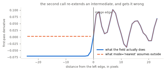
The gap between the two curves outside the edge is what the second call integrates over, and it is why the border band is wrong.
A single gaussian_filter call touches each axis once, so it is exact — a
separable 2-D Gaussian is bit-identical to the padded 2-D convolution.
Separability is innocent.
The two calls
_hessian_matrix_with_gaussian never asks for a second derivative directly. It
asks for a first derivative twice, and the source says why, immediately
above the loop:
    # Apply two successive first order Gaussian derivative operations, as
    # detailed in:
    # https://dsp.stackexchange.com/questions/78280/are-scipy-second-order-gaussian-derivatives-correct
That page is the second-derivative aliasing of section 3, reported by someone who met it in practice. The workaround is sound as far as it goes: a first-derivative kernel is odd, so it sums to zero by symmetry however coarsely it is sampled, and composing two of them never asks SciPy for the even kernel that leaks. The subsection on other libraries returns to what else that page contains.
What it costs is this section. Two calls, each at sigma / sqrt(2):
One call per axis, on the image.
order=[1, 0]givesd/drof the smoothed image andorder=[0, 1]givesd/dc. For a 2-D image that is two calls, producing two gradient fields.One call per element, on a gradient field. Each Hessian entry takes one of those fields and differentiates it again along one axis.
Hrrisd/drapplied to thed/drfield,Hccisd/dcapplied to thed/dcfield, andHrcisd/dcapplied to thed/drfield.
Written out, with nothing hidden:
scaled = SIGMA / np.sqrt(2)
filter_kwargs = dict(mode=MODE, truncate=8)

# Call 1: a first derivative along each axis, over the whole image.
grad_r = ndi.gaussian_filter(IMG, scaled, order=[1, 0], **filter_kwargs)
grad_c = ndi.gaussian_filter(IMG, scaled, order=[0, 1], **filter_kwargs)

# Call 2: a second first derivative, applied to one of those fields.
by_hand = [
    ndi.gaussian_filter(grad_r, scaled, order=[1, 0], **filter_kwargs),   # Hrr
    ndi.gaussian_filter(grad_r, scaled, order=[0, 1], **filter_kwargs),   # Hrc
    ndi.gaussian_filter(grad_c, scaled, order=[0, 1], **filter_kwargs),   # Hcc
]

shipped = hessian_matrix(IMG, sigma=SIGMA, mode=MODE,
                         use_gaussian_derivatives=True)
for name, mine, theirs in zip(("Hrr", "Hrc", "Hcc"), by_hand, shipped):
    print(f"{name}: reproduces hessian_matrix exactly: "
          f"{np.array_equal(mine, theirs)}")
Hrr: reproduces hessian_matrix exactly: True
Hrc: reproduces hessian_matrix exactly: True
Hcc: reproduces hessian_matrix exactly: True
Each of those calls is itself two one-dimensional passes, so one 2-D Hessian entry costs four passes arranged as two calls. The passes are not the problem; the calls are. A boundary extension is applied per call, so every axis is extended twice, and on the second occasion it is extended from an array the first call has already smoothed along that axis. Cropping threw information away; re-padding invents a replacement.
That also explains the ordering difference. Hrc above runs d/dr and then
d/dc. Asking for order='xy' runs d/dc and then d/dr, which re-extends a
different intermediate, so the two disagree wherever the extension is felt.
8. There is a right answer, and no element has it
Pad once by the rule mode names, filter with a wide margin, then crop. In
that construction the two orders agree to 1e-17, so it defines the quantity
both are approximating.
def reference(image, sigma, mode=MODE, npmode="edge"):
    """The Hessian of the smoothed, once-extended image."""
    trunc = 8 if sigma > 1 else 100
    pad = 2 * int(trunc * sigma / np.sqrt(2) + 0.5) + 1
    big = np.pad(image, pad, mode=npmode)
    H = hessian_matrix(big, sigma=sigma, mode=mode, use_gaussian_derivatives=True)
    return [h[pad:-pad, pad:-pad] for h in H]


ref = reference(IMG, SIGMA)
cur = hessian_matrix(IMG, sigma=SIGMA, mode=MODE, use_gaussian_derivatives=True)

names = ["Hrr (diagonal)", "Hrc (mixed)", "Hcc (diagonal)"]
fig, axes = plt.subplots(1, 3, figsize=(9.6, 2.8))
for ax, name, c, r in zip(axes, names, cur, ref):
    d = np.abs(c - r)
    im = show(ax, d, f"{name}\nmax {d.max():.1e}, {d.max()/np.abs(r).max():.0%} of range")
    fig.colorbar(im, ax=ax, fraction=0.046)
fig.suptitle("every element is wrong at the border, not just the mixed one", y=1.04)
fig.tight_layout()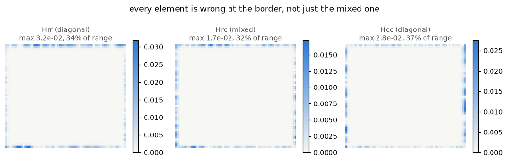
for name, c, r in zip(names, cur, ref):
    d = np.abs(c - r)
    print(f"{name:<16} max {d.max():.3e}  relative {d.max()/np.abs(r).max():6.1%}"
          f"   interior {d[20:-20, 20:-20].max():.2e}")
Hrr (diagonal) max 3.195e-02 relative 34.0% interior 0.00e+00
Hrc (mixed) max 1.724e-02 relative 31.5% interior 0.00e+00
Hcc (diagonal) max 2.756e-02 relative 36.7% interior 0.00e+00
The interior is exact. The defect is confined to a border band, and inside that band it reaches about a third of the signal.
radius = int(8 * SIGMA / np.sqrt(2) + 0.5)
profile = np.abs(cur[1] - ref[1]).max(axis=0)

fig, ax = plt.subplots(figsize=(6.4, 2.6))
ax.semilogy(np.arange(len(profile)), np.maximum(profile, 1e-18), color=C_ONE, lw=2)
for edge in (radius, len(profile) - 1 - radius):
    ax.axvline(edge, color=C_TWO, lw=1.5, ls="--")
ax.annotate("one kernel radius", (radius, profile.max()), xytext=(6, -4),
            textcoords="offset points", fontsize=8, color=C_TWO)
ax.set_xlabel("column", fontsize=8, color=MUTED)
ax.set_ylabel("max error in that column", fontsize=8, color=MUTED)
ax.tick_params(labelsize=8, colors=MUTED)
for s in ("top", "right"):
    ax.spines[s].set_visible(False)
for s in ("left", "bottom"):
    ax.spines[s].set_color(GRID)
ax.set_title("the error stops exactly one kernel radius in")
fig.tight_layout()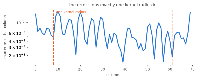
9. It reaches the ridge filters
frangi, sato, meijering and hessian all call hessian_matrix with
use_gaussian_derivatives=True.
Two details matter for making the comparison mean anything. The ridge filters
default to mode='reflect', so the once-extended reference has to be built with
the matching numpy rule, not with edge; and their default sigmas start at
1, where hessian_matrix raises truncate to 100, so the margin has to exceed
one hundred pixels rather than the forty a truncate = 8 kernel would need.
Both are easy to get wrong, and either one on its own produces a difference that
has nothing to do with the defect.
That truncate = 100 is the first of several appearances after section 3. It is
the small-sigma FIR-width guard described there: it does not repair the failed
moments, but it does force every pad-once construction to clear a ~100-pixel
margin. It turns up again as a cost in Fix B, as the reason Fix A is slow at
sigma = 0.5, and finally in Fix C, which removes the reason for keeping it.
photo = ski.util.img_as_float(ski.data.camera())[::2, ::2]
PAD = 110                                  # > truncate 100 * sigma 1
RIDGE = dict(mode="nearest")               # matches np.pad(..., mode='edge')
padded = np.pad(photo, PAD, mode="edge")

RIDGE_FILTERS = [("frangi", frangi), ("sato", sato),
                 ("meijering", meijering), ("hessian", hessian)]

fig, axes = plt.subplots(3, 4, figsize=(10.5, 7.6))
for col, (name, f) in enumerate(RIDGE_FILTERS):
    direct = f(photo, **RIDGE)
    ref_out = f(padded, **RIDGE)[PAD:-PAD, PAD:-PAD]
    diff = np.abs(direct - ref_out)
    show(axes[0, col], direct, f"{name}, as computed")
    show(axes[1, col], ref_out, "with the border handled once")
    im = show(axes[2, col], diff,
              f"difference, {diff.max()/max(np.abs(ref_out).max(), 1e-12):.0%} of range")
    fig.colorbar(im, ax=axes[2, col], fraction=0.046)
fig.suptitle("the border defect, end to end", y=1.01)
fig.tight_layout()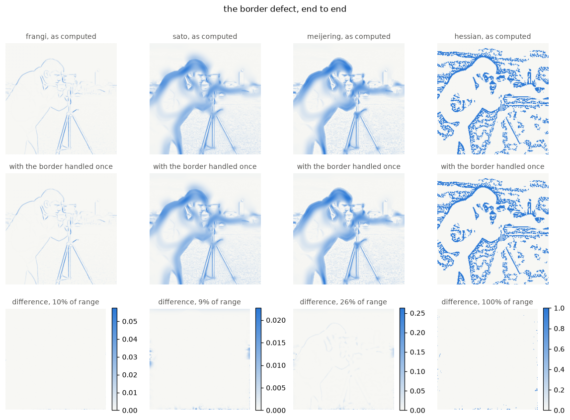
def ridge_border_error(label):
    """Each ridge filter against itself on a once-extended image."""
    print(f"{label}")
    for name, f in RIDGE_FILTERS:
        a = f(photo, **RIDGE)
        b = f(padded, **RIDGE)[PAD:-PAD, PAD:-PAD]
        d = np.abs(a - b)
        print(f"   {name:<10} max {d.max():.3e} "
              f"({d.max()/max(np.abs(b).max(), 1e-12):6.1%} of range)"
              f"   30 px in: {d[30:-30, 30:-30].max():.2e}")


ridge_border_error("as shipped")
as shipped
frangi max 5.749e-02 ( 9.9% of range) 30 px in: 4.52e-11
sato max 2.268e-02 ( 9.3% of range) 30 px in: 1.52e-07
meijering max 2.630e-01 ( 26.3% of range) 30 px in: 3.27e-02
hessian max 1.000e+00 (100.0% of range) 30 px in: 6.82e-15
hessian flips completely at the border. meijering also moves in the
interior, because it normalises by a global maximum that the border artefact
distorts.
10. Three candidate fixes
Fix A: compute every element in one call
Section 7 named the cause exactly: a boundary extension is applied per call,
so any element built from two calls extends some axis twice. The remedy follows
from the cause. Ask scipy.ndimage.gaussian_filter for the whole derivative in
one call, at the full sigma, using the order vector to say which axes to
differentiate and how many times:
| element | order | axes touched |
|---|---|---|
Hrr | [2, 0] | axis 0 once, at second order |
Hrc | [1, 1] | each axis once, at first order |
Hcc | [0, 2] | axis 1 once, at second order |
def one_call(image, sigma, mode=MODE, order="rc"):
    """Every Hessian element from a single `gaussian_filter` call, at full sigma."""
    trunc = 8 if sigma > 1 else 100
    kw = dict(mode=mode, truncate=trunc)
    orders = ([2, 0], [1, 1], [0, 2])
    if order == "xy":
        orders = orders[::-1]
    return [ndi.gaussian_filter(image, sigma, order=o, **kw) for o in orders]
The mixed element [1, 1] is the easy half of this, and it is uncontroversial:
it differentiates each axis once, so no axis is touched twice. The diagonals are
the question, because order=2 is what the code comment in corner.py steers
away from, citing scipy’s second-order Gaussian derivatives. That claim is
testable, so test it rather than assume it.
Every element becomes exact. Against a pad-once reference built the same way, the difference is not merely small — it is zero to the last bit.
def padded_reference(f, image, sigma, npmode="edge", **kw):
    """Run `f` on a generously extended image, then crop back."""
    trunc = 8 if sigma > 1 else 100
    pad = 2 * int(trunc * sigma + 0.5) + 1
    big = np.pad(image, pad, mode=npmode)
    return [e[pad:-pad, pad:-pad] for e in f(big, sigma, **kw)]


one = one_call(IMG, SIGMA)
one_ref = padded_reference(one_call, IMG, SIGMA)
one_scale = max(np.abs(e).max() for e in one_ref)

print(f"{'element':<18}{'two calls, as shipped':>24}{'one call':>12}")
for name, c, o, r, orf in zip(names, cur, one, ref, one_ref):
    print(f"{name:<18}{np.abs(c - r).max() / np.abs(r).max():>23.1%}"
          f"{np.abs(o - orf).max() / one_scale:>12.1e}")
element two calls, as shipped one call
Hrr (diagonal) 34.0% 0.0e+00
Hrc (mixed) 31.5% 0.0e+00
Hcc (diagonal) 36.7% 0.0e+00
The order ambiguity disappears rather than shrinking. [2, 0] and
[0, 2] are each other’s mirror and [1, 1] is its own, so relabelling the
axes permutes the three results and changes nothing else.
def order_disagreement(f):
    """Relative disagreement between order='rc' and order='xy'."""
    rc, xy = f(order="rc"), f(order="xy")
    sc = max(np.abs(e).max() for e in rc)
    return max(np.abs(a - b).max() for a, b in zip(rc, xy[::-1])) / sc


shipped = lambda order: hessian_matrix(IMG, sigma=SIGMA, mode=MODE, order=order,
                                       use_gaussian_derivatives=True)
print("order='rc' against order='xy', for the same quantity")
print(f"   two calls, as shipped : {order_disagreement(shipped):.2e}")
print(f"   one call              : "
      f"{order_disagreement(lambda order: one_call(IMG, SIGMA, order=order)):.2e}")
order='rc' against order='xy', for the same quantity
two calls, as shipped : 4.33e-01
one call : 0.00e+00
In the interior it is more accurate, not less. This is the measurement that
answers the code comment. Against the analytic Hessian of section 3, one call
beats two from about sigma = 0.7 upwards, usually by an order of magnitude,
and from about sigma = 0.75 it beats finite differences as well.
print(f"{'sigma':>6}{'finite diffs':>15}{'two calls':>12}{'one call':>12}{'best':>14}")
for sigma in (0.5, 0.6, 0.7, 0.75, 0.8, 0.9, 1.0, 1.5, 3.0):
    fd = relative_error(hessian_matrix(blob, sigma=sigma, mode="nearest",
                                       use_gaussian_derivatives=False), sigma)
    tc = relative_error(hessian_matrix(blob, sigma=sigma, mode="nearest",
                                       use_gaussian_derivatives=True), sigma)
    oc = relative_error(one_call(blob, sigma, mode="nearest"), sigma)
    best = min([(fd, "finite"), (tc, "two calls"), (oc, "one call")])[1]
    print(f"{sigma:>6}{fd:>14.2%}{tc:>12.2%}{oc:>12.2%}{best:>14}")
sigma finite diffs two calls one call best
0.5 106.53% 100.38% 229.77% two calls
0.6 106.47% 101.83% 121.24% two calls
0.7 106.43% 104.09% 108.05% two calls
0.75 106.41% 105.17% 107.12% two calls
0.8 106.38% 105.88% 106.86% two calls
   0.9       106.34%     106.51%     106.74%        finite
   1.0       106.29%     106.65%     106.70%        finite
   1.5       106.07%     106.50%     106.50%        finite
   3.0       107.41%     107.63%     107.63%        finite
So the comment is right about the direction of the risk and wrong about where
it bites. Above about sigma = 0.7 the extra pass costs more accuracy than the
harder kernel does, and the crossover against finite differences moves from
about sigma = 0.85 down to about sigma = 0.73. Below sigma = 0.65 one call
is far worse — 950% against 92% at sigma = 0.5.
That last figure deserves more than a shrug, because the two schemes do not fail
in the same way. Two tests separate them: a constant image, whose Hessian is
zero everywhere, and a quadratic ramp f = r**2 / 2, whose Hrr is 1
everywhere.
const = np.ones((40, 40))
ramp = np.repeat((np.arange(400.0)[:, None] - 200) ** 2 / 2, 8, axis=1)
middle = (200, 4)


def two_calls(image, sigma, mode=MODE):
    """The shipped scheme, written out."""
    trunc = 8 if sigma > 1 else 100
    kw = dict(mode=mode, truncate=trunc)
    scaled = sigma / np.sqrt(2)
    grad = ndi.gaussian_filter(image, scaled, order=[1, 0], **kw)
    return ndi.gaussian_filter(grad, scaled, order=[1, 0], **kw)


print(f"{'':7}{'constant, want 0':>28}{'quadratic ramp, want 1':>32}")
print(f"{'sigma':>7}{'two calls':>14}{'one call':>14}{'two calls':>16}{'one call':>16}")
for sigma in (0.5, 0.7, 1.0, 1.5):
    print(f"{sigma:>7}"
          f"{two_calls(const, sigma)[20, 20]:>14.4f}"
          f"{one_call(const, sigma)[0][20, 20]:>14.4f}"
          f"{two_calls(ramp, sigma)[middle]:>16.4f}"
          f"{one_call(ramp, sigma)[0][middle]:>16.4f}")
constant, want 0 quadratic ramp, want 1
sigma two calls one call two calls one call
0.5 0.0000 -0.5598 0.0799 1.3408
0.7 0.0000 -0.0050 0.7205 1.0175
1.0 0.0000 -0.0000 0.9959 1.0000
1.5 0.0000 -0.0000 1.0000 1.0000
The shipped scheme suffers gain collapse. At sigma = 0.5 it reports about
eight per cent of the true curvature — badly wrong in size, but the sign is
right, the structure is right, and it returns exactly zero on a constant. A
first-derivative kernel is odd, so it sums to zero by symmetry whatever the
sampling does to it.
One call has a DC leak, which is worse in kind. Its order=2 kernel is
even, and nothing forces the sampled version to sum to zero. At sigma = 0.5
it sums to -0.56, so the operator responds to absolute brightness: a flat
bright region reads as strongly curved, and the reported curvature depends on
what you added to the image rather than on its shape.
Those are the failed moments from section 3 — the same aliasing, now felt as a defect of Fix A rather than of the shipped two-call route. The second moment is wrong at the same time; both fail together because the continuous kernel varies faster than the grid can follow.
print("moments of the order=2 kernel (truncate as shipped); "
      "need sum 0 and sum k*x**2/2 = 1")
print(f"{'sigma':>7}{'sum':>14}{'sum k*x**2/2':>16}")
for sigma in (0.4, 0.5, 0.7, 1.0, 1.5):
    x, k = gaussian_taps(sigma, 2, 8 if sigma > 1 else 100)
    print(f"{sigma:>7}{k.sum():>14.2e}{(k * x**2).sum() / 2:>16.4f}")
moments of the order=2 kernel (truncate as shipped); need sum 0 and sum k*x**2/2 = 1
sigma sum sum k*x**2/2
0.4 -3.09e+00 1.3273
0.5 -5.60e-01 1.3408
0.7 -4.97e-03 1.0175
1.0 -2.11e-07 1.0000
1.5 -8.37e-16 1.0000
It is not slower. Six one-dimensional passes replace ten, against kernels
sqrt(2) wider.
import time


def best_of(f, n=7):
    """Smallest wall-clock time over `n` runs, after one warm-up."""
    f()
    times = []
    for _ in range(n):
        t0 = time.perf_counter()
        f()
        times.append(time.perf_counter() - t0)
    return min(times)


print(f"{'sigma':>6}{'truncate':>10}{'two calls':>13}{'one call':>12}{'ratio':>8}")
for sigma in (0.5, 1.0, 1.5, 3.0, 6.0):
    t_two = best_of(lambda: hessian_matrix(photo, sigma=sigma, mode=MODE,
                                           use_gaussian_derivatives=True))
    t_one = best_of(lambda: one_call(photo, sigma))
    print(f"{sigma:>6}{8 if sigma > 1 else 100:>10}{t_two * 1e3:>10.1f} ms"
          f"{t_one * 1e3:>10.1f} ms{t_one / t_two:>7.2f}x")
sigma truncate two calls one call ratio
0.5 100 15.3 ms 17.7 ms 1.15x
   1.0       100      34.6 ms      26.0 ms   0.75x
   1.5         8       5.5 ms       3.3 ms   0.60x
3.0 8 8.0 ms 7.4 ms 0.92x
6.0 8 14.4 ms 10.9 ms 0.76x
It is faster from sigma = 1 upwards, and slower at sigma = 0.5 only because
the truncate = 100 guard then makes the full-sigma kernel the wider one.
That width is not required by Fix A itself: Fix C shows the guard can go, and
removing it turns this row around.
It generalises to N dimensions unchanged. The order vector carries a 2 on
the diagonal and two 1s off it, whatever the dimension.
def one_call_nd(image, sigma, mode=MODE):
    """The same rule, written for any number of dimensions."""
    trunc = 8 if sigma > 1 else 100
    kw = dict(mode=mode, truncate=trunc)
    out = []
    for a in range(image.ndim):
        for b in range(a, image.ndim):
            orders = [0] * image.ndim
            orders[a] += 1
            orders[b] += 1
            out.append(ndi.gaussian_filter(image, sigma, order=orders, **kw))
    return out


vol = np.random.default_rng(3).random((24, 26, 28))
P3 = 40
crop = (slice(P3, -P3),) * 3
big3 = np.pad(vol, P3, mode="edge")

two_3d = hessian_matrix(vol, sigma=SIGMA, mode=MODE, use_gaussian_derivatives=True)
two_3d_ref = [e[crop] for e in hessian_matrix(big3, sigma=SIGMA, mode=MODE,
                                              use_gaussian_derivatives=True)]
one_3d = one_call_nd(vol, SIGMA)
one_3d_ref = [e[crop] for e in one_call_nd(big3, SIGMA)]
sc3 = max(np.abs(e).max() for e in one_3d_ref)

print(f"3-D volume, {len(two_3d)} elements, worst border error")
print(f"   two calls : "
      f"{max(np.abs(a - b).max() for a, b in zip(two_3d, two_3d_ref)) / sc3:.1%}")
print(f"   one call  : "
      f"{max(np.abs(a - b).max() for a, b in zip(one_3d, one_3d_ref)) / sc3:.1e}")
3-D volume, 6 elements, worst border error
two calls : 49.1%
one call : 0.0e+00
End to end, three of the four ridge filters become exact. The ridge filters
import hessian_matrix from the corner module when they are called, so
replacing it there runs the whole pipeline on Fix A.
import importlib
import sys
from unittest import mock

package = sys.modules[frangi.__module__].__package__.rsplit(".", 1)[0]
corner_mod = importlib.import_module(f"{package}.feature.corner")


def as_hessian_matrix(rule):
    """Wrap a Hessian rule in the `hessian_matrix` signature, ready to patch in."""
    def replacement(image, sigma=1, mode="reflect", cval=0, order="rc",
                    use_gaussian_derivatives=True):
        return rule(ski.util.img_as_float(image), sigma, mode=mode)
    return replacement


with mock.patch.object(corner_mod, "hessian_matrix", as_hessian_matrix(one_call_nd)):
    ridge_border_error("with Fix A")
with Fix A
frangi max 0.000e+00 ( 0.0% of range) 30 px in: 0.00e+00
sato max 0.000e+00 ( 0.0% of range) 30 px in: 0.00e+00
meijering max 3.279e-02 ( 3.3% of range) 30 px in: 3.26e-02
hessian max 0.000e+00 ( 0.0% of range) 30 px in: 0.00e+00
frangi, sato and hessian go to zero exactly — not to a small residue.
meijering drops from 26.3% to 3.3%, and what is left is the interior figure,
unchanged: it normalises by a global maximum, and cropping a border band shifts
that maximum. That is a separate defect in meijering, which the border fix
exposes rather than causes.
Fix B: pad once inside the function
Extend the image by the rule mode names, run the existing scheme, crop. Every
element becomes exact. This was the obvious fix before Fix A was measured, and
it reaches the same place by paying for it: the second extension is still wrong,
so the padding exists to push it far enough away to be cropped off.
import time

# Timed on the 256x256 photograph, not the small test array: the padding cost
# is relative to image size, so a toy array badly overstates it.
print(f"{'sigma':>6}{'pad':>6}{'current':>12}{'padded':>10}{'cost':>8}")
for sigma in (0.5, 1.0, 1.5, 3.0):
    t0 = time.perf_counter()
    hessian_matrix(photo, sigma=sigma, mode=MODE, use_gaussian_derivatives=True)
    t1 = time.perf_counter()
    reference(photo, sigma)
    t2 = time.perf_counter()
    trunc = 8 if sigma > 1 else 100
    pad = 2 * int(trunc * sigma / np.sqrt(2) + 0.5) + 1
    print(f"{sigma:>6}{pad:>6}{(t1-t0)*1e3:>10.1f} ms{(t2-t1)*1e3:>8.1f} ms"
          f"{(t2-t1)/(t1-t0):>7.1f}x")
sigma pad current padded cost
0.5 71 18.2 ms 38.2 ms 2.1x
   1.0   143      39.6 ms   160.8 ms    4.1x
   1.5    17       6.8 ms     5.1 ms    0.7x
   3.0    35       9.1 ms    10.6 ms    1.2x
The cost is modest above sigma = 1. Below it the function sets
truncate = 100, and the padding has to clear that support, so the margin
becomes enormous — 143 pixels at sigma = 1. That width is the aliasing guard
from section 3, not a moment fix; Fix C removes the reason for keeping the
guard, which removes most of this cost with it.
Fix C: correct the kernel, so Fix A works at every scale
Fix A’s only weakness is the small-sigma aliasing of section 3, stated there
as two failed moment conditions. A discrete second-derivative operator has to
annihilate constants and reproduce quadratics:
    sum(k)             ==  0        no response to a constant
    sum(k * x**2) / 2  ==  1        exact on f = x**2 / 2
Imposing both on the sampled kernel is a local consistency repair, and it takes two lines. It is not Lindeberg’s discrete Gaussian derivative construction: that construction smooths with the discrete Bessel-kernel scale space and then applies small-support central differences.
def corrected_taps(sigma, order, trunc=8):
    """Gaussian derivative taps with the discrete moments repaired."""
    x, g = gaussian_taps(sigma, 0, trunc)
    _, k = gaussian_taps(sigma, order, trunc)
    if order == 0:
        return x, g
    if order == 1:
        return x, k / (k * x).sum()             # exact on f = x
    k = k - k.sum() * g                         # annihilate constants
    return x, k / ((k * x**2).sum() / 2)        # exact on f = x**2 / 2
There is a choice in the first correction that turns out to matter more than it
looks. The obvious way is to subtract k.sum() / k.size from every tap, which
also makes the kernel sum to zero, and it is what DIPlib and VIGRA both do. The
version above instead subtracts a multiple of the Gaussian itself. The two are
identical in total and differ only in where they put it.
Spreading it evenly is correct at a sane kernel width and fails at
truncate = 100: with 141 taps at sigma = 0.7 and about four of them carrying
the operator, an even correction lays a wide plateau under a one-pixel
derivative. Spreading it along g is insensitive to the window, which is why
this notebook uses it — but that robustness is only needed because of the
truncate = 100 guard, and the subsection on other libraries returns to the point.
def flat_corrected_taps(sigma, order, trunc=8):
    """Even subtraction: what DIPlib and VIGRA do, at their own kernel widths."""
    x, k = gaussian_taps(sigma, order, trunc)
    if order != 2:
        return corrected_taps(sigma, order, trunc)
    k = k - k.sum() / k.size
    return x, k / ((k * x**2).sum() / 2)


def with_taps(taps_of, image, sigma, mode=MODE, trunc=8):
    """Build the three elements from whichever tap rule is passed."""
    taps = {o: taps_of(sigma, o, trunc)[1] for o in (0, 1, 2)}
    sep = lambda a, b: ndi.correlate1d(
        ndi.correlate1d(image, taps[a], axis=0, mode=mode), taps[b], axis=1, mode=mode)
    return [sep(2, 0), sep(1, 1), sep(0, 2)]


print(f"{'sigma':>7}{'taps':>7}{'corrected along g':>20}{'corrected flat':>17}")
for sigma in (0.5, 0.7, 1.0):
    trunc = 8 if sigma > 1 else 100          # shipped guard, not a moment fix
    n = 2 * int(trunc * sigma + 0.5) + 1
    along = relative_error(
        with_taps(corrected_taps, blob, sigma, mode="nearest", trunc=trunc), sigma)
    flat = relative_error(
        with_taps(flat_corrected_taps, blob, sigma, mode="nearest", trunc=trunc), sigma)
    print(f"{sigma:>7}{n:>7}{along:>19.2%}{flat:>17.2%}")
sigma taps corrected along g corrected flat
0.5 101 106.94% 100.38%
0.7 141 106.84% 101.13%
1.0 201 106.70% 106.69%
What the correction does, in pictures
The two moment conditions are easier to believe once you see the kernel they
act on. At sigma = 1.5 the sampled second derivative is a smooth,
well-resolved curve; at sigma = 0.5 it is three or four significant taps
trying to represent a function that swings through its whole range inside one
pixel.
fig, axes = plt.subplots(1, 2, figsize=(9.0, 2.9))
for ax, sigma in zip(axes, (1.5, 0.5)):
    x, k = gaussian_taps(sigma, 2, trunc=8)
    dense = np.linspace(x.min(), x.max(), 2001)
    g = np.exp(-(dense**2) / (2 * sigma**2))
    g /= np.exp(-(x**2) / (2 * sigma**2)).sum()
    ax.plot(dense, g * ((dense**2 - sigma**2) / sigma**4), color=GRID, lw=2,
            zorder=1, label="the continuous kernel")
    ax.plot(x, k, "o", color=C_ONE, markersize=6, zorder=3, label="what is sampled")
    ax.vlines(x, 0, k, color=C_ONE, lw=1.2, zorder=2)
    ax.axhline(0, color=MUTED, lw=0.8)
    ax.set_xlim(-5 * sigma, 5 * sigma)
    ax.set_title(f"sigma = {sigma}: taps sum to {k.sum():+.3f}")
    ax.tick_params(labelsize=8, colors=MUTED)
    for s in ("top", "right"):
        ax.spines[s].set_visible(False)
    for s in ("left", "bottom"):
        ax.spines[s].set_color(GRID)
axes[0].legend(frameon=False, fontsize=8)
fig.suptitle("the same operator, sampled well and sampled badly", y=1.03)
fig.tight_layout()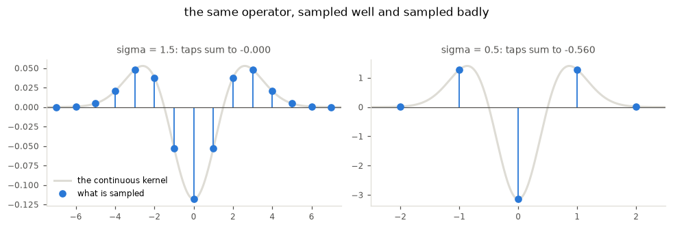
The continuous curve integrates to zero — the positive flanks exactly cancel the
negative well. The sampled version only inherits that when the samples are dense
enough to see both. At sigma = 0.5 they are not, the cancellation fails, and
the sum is what is left over.
That leftover is the whole defect, and it is visible directly as a response to a flat image.
flat_patch = np.ones((40, 40))
ramp = np.repeat((np.arange(400.0)[:, None] - 200) ** 2 / 2, 8, axis=1)

fig, axes = plt.subplots(1, 2, figsize=(9.0, 2.9))
sigmas = np.linspace(0.3, 1.6, 40)
for taps_of, name, colour in ((gaussian_taps, "as sampled", C_TWO),
                              (corrected_taps, "corrected", C_ONE)):
    dc = [with_taps(taps_of, flat_patch, s, mode="nearest")[0][20, 20] for s in sigmas]
    quad = [with_taps(taps_of, ramp, s, mode="nearest")[0][200, 4] for s in sigmas]
    axes[0].plot(sigmas, dc, color=colour, lw=2, label=name)
    axes[1].plot(sigmas, quad, color=colour, lw=2, label=name)
for ax, target, title in ((axes[0], 0.0, "response to a constant (want 0)"),
                          (axes[1], 1.0, "response to r**2 / 2 (want 1)")):
    ax.axhline(target, color=MUTED, lw=1, ls="--")
    ax.set_xlabel("sigma", fontsize=8, color=MUTED)
    ax.set_title(title)
    ax.tick_params(labelsize=8, colors=MUTED)
    for s in ("top", "right"):
        ax.spines[s].set_visible(False)
    for s in ("left", "bottom"):
        ax.spines[s].set_color(GRID)
axes[0].legend(frameon=False, fontsize=8)
fig.suptitle("the two conditions, as functions of scale", y=1.03)
fig.tight_layout()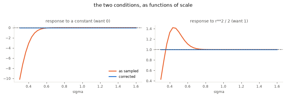
Above sigma = 1 the sampled kernel satisfies both conditions on its own and
the correction changes nothing. Below it the sampled curve leaves both, fast,
while the corrected one sits on the target by construction.
Where the correction is put matters as much as its size. Both variants
remove the same total, k.sum(). They differ only in how they spread it, and
that is the whole distance between 0.67% and 96%.
fig, axes = plt.subplots(1, 2, figsize=(9.6, 3.0))
for ax, trunc in zip(axes, (8, 100)):
    x, raw = gaussian_taps(0.5, 2, trunc=trunc)
    _, g0 = gaussian_taps(0.5, 0, trunc=trunc)
    # Cumulative mass of each correction, so width is what the eye reads.
    ax.plot(x, np.cumsum(-raw.sum() * g0), color=C_ONE, lw=2,
            label="along g: all of it under the operator")
    ax.plot(x, np.cumsum(np.full_like(x, -raw.sum() / raw.size)), color=C_TWO,
            lw=2, label="flat: accumulated across the whole window")
    ax.axvspan(-2, 2, color=GRID, alpha=0.6, zorder=0)
    ax.annotate("operator\nsupport", (0, 0), xytext=(0, 6), textcoords="offset points",
                ha="center", fontsize=7, color=MUTED)
    ax.set_xlim(x.min(), x.max())
    ax.set_title(f"sigma = 0.5, truncate = {trunc}  ({raw.size} taps, "
                 f"reach +/-{int(x.max())} px)")
    ax.set_xlabel("pixels from centre", fontsize=8, color=MUTED)
    ax.tick_params(labelsize=8, colors=MUTED)
    for s in ("top", "right"):
        ax.spines[s].set_visible(False)
    for s in ("left", "bottom"):
        ax.spines[s].set_color(GRID)
axes[0].set_ylabel("cumulative correction", fontsize=8, color=MUTED)
axes[0].legend(frameon=False, fontsize=7, loc="upper left")
fig.suptitle("the same total mass, delivered over two very different widths",
             y=1.03)
fig.tight_layout()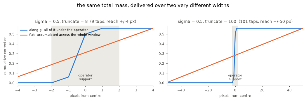
Both curves climb to the same final value: both variants remove exactly
k.sum(). The difference is where they collect it. The along-g correction
has finished by two pixels out — it lies inside the operator’s own support, the
shaded band. The flat correction accrues in a straight line all the way to the
window edge, so most of its mass sits where the operator has none.
That is why the height of the plateau is the wrong thing to look at. At
truncate = 100 the shelf is only 0.0055 tall and looks negligible, but it is
101 taps wide, and a wide shallow shelf convolved with an image is a local mean
over 101 pixels. Adding a local mean to a one-pixel second derivative is the
96%. At truncate = 8 the window is 9 taps, the shelf is barely wider than the
operator, and there is almost nothing to add.
The along-g correction has no such dependence, because it is shaped like the
operator it corrects. That is worth stating as the design rule: remove the
leaked constant using the same envelope that leaked it.
Both elements of the Hessian then come from one call each, exactly as in Fix A, except that the taps are supplied rather than requested by name. Two 1-D passes along different axes still commute with the boundary extension, so section 7’s guarantee is untouched.
def fix_c(image, sigma, mode=MODE, trunc=8, order="rc"):
    """Fix A, with the corrected kernels and no `truncate = 100` guard."""
    taps = {o: corrected_taps(sigma, o, trunc)[1] for o in (0, 1, 2)}

    def sep(first, second):
        out = ndi.correlate1d(image, taps[first], axis=0, mode=mode)
        return ndi.correlate1d(out, taps[second], axis=1, mode=mode)

    out = [sep(2, 0), sep(1, 1), sep(0, 2)]
    return out[::-1] if order == "xy" else out
It removes the small-sigma cost rather than trading it away.
print(f"{'sigma':>6}{'finite':>10}{'two calls':>12}{'Fix A':>10}{'Fix C':>10}")
for sigma in (0.4, 0.5, 0.6, 0.7, 0.75, 0.8, 0.9, 1.0, 1.5, 3.0):
    print(f"{sigma:>6}"
          f"{relative_error(hessian_matrix(blob, sigma=sigma, mode='nearest', use_gaussian_derivatives=False), sigma):>9.2%}"
          f"{relative_error(hessian_matrix(blob, sigma=sigma, mode='nearest', use_gaussian_derivatives=True), sigma):>12.2%}"
          f"{relative_error(one_call(blob, sigma, mode='nearest'), sigma):>10.2%}"
          f"{relative_error(fix_c(blob, sigma, mode='nearest'), sigma):>10.2%}")
sigma finite two calls Fix A Fix C
0.4 106.60% 100.01% 794.59% 106.94%
0.5 106.53% 100.38% 229.77% 106.94%
0.6 106.47% 101.83% 121.24% 106.90%
0.7 106.43% 104.09% 108.05% 106.84%
0.75 106.41% 105.17% 107.12% 106.81%
0.8 106.38% 105.88% 106.86% 106.79%
0.9 106.34% 106.51% 106.74% 106.74%
1.0 106.29% 106.65% 106.70% 106.70%
1.5 106.07% 106.50% 106.50% 106.50%
3.0 107.41% 107.63% 107.63% 107.63%
blob is a very smooth test object, which flatters finite differences. A
sinusoid of known wavelength is a harder and more honest test, because the
smoothed answer is analytic at every frequency and the frequency is a knob.
N = 200
si, sj = np.indices((N, N), dtype=float)
INNER = (slice(20, -20),) * 2

print("interior error on f = cos(2*pi*r/L), at sigma = 0.5")
print(f"{'L, pixels':>11}{'finite':>10}{'two calls':>12}{'Fix A':>10}{'Fix C':>10}")
for L in (40, 20, 10, 8, 5, 4):          # each divides N, so mode='wrap' is exact
    w = 2 * np.pi / L
    wave = np.cos(w * si)
    truth = -(w**2) * np.exp(-(w**2) * 0.25 / 2) * np.cos(w * si)
    scale = (w**2) * np.exp(-(w**2) * 0.25 / 2)

    def miss(got):
        return np.abs(got[INNER] - truth[INNER]).max() / scale

    smooth = ndi.gaussian_filter(wave, 0.5, mode="wrap")
    fd = np.gradient(np.gradient(smooth)[0])[0]
    print(f"{L:>11}{miss(fd):>9.2%}"
          f"{miss(two_calls(wave, 0.5, mode='wrap')):>12.2%}"
          f"{miss(one_call(wave, 0.5, mode='wrap')[0]):>10.2%}"
          f"{miss(fix_c(wave, 0.5, mode='wrap')[0]):>10.2%}")
interior error on f = cos(2*pi*r/L), at sigma = 0.5
L, pixels finite two calls Fix A Fix C
40 0.78% 92.05% 2309.95% 0.07%
20 3.08% 92.17% 608.71% 0.30%
10 11.83% 92.65% 184.64% 1.20%
8 17.95% 93.00% 134.60% 1.89%
          5   40.55%      94.42%    83.79%     4.93%
          4   56.63%      95.59%    75.33%     7.82%
Finite differences run from 0.8% to 57% at a fixed sigma, purely with image
content. Their apparent advantage below sigma = 0.85 is a property of the
smooth blob, not of the method, which is worth knowing before treating them as
the safe fallback at small scale.
Everything Fix A won is kept.
print(f"{'sigma':>6}{'border vs pad-once':>21}{'order rc vs xy':>17}"
      f"{'response to a constant':>25}")
for sigma in (0.4, 0.5, 0.7, 1.0, 1.5, 3.0):
    pad = 2 * int(8 * sigma + 0.5) + 1
    direct = fix_c(IMG, sigma)
    padded_ref = [e[pad:-pad, pad:-pad]
                  for e in fix_c(np.pad(IMG, pad, mode="edge"), sigma)]
    sc = max(np.abs(e).max() for e in padded_ref)
    swapped = fix_c(IMG, sigma, order="xy")[::-1]
    print(f"{sigma:>6}"
          f"{max(np.abs(a - b).max() for a, b in zip(direct, padded_ref)) / sc:>20.1e}"
          f"{max(np.abs(a - b).max() for a, b in zip(direct, swapped)) / sc:>17.1e}"
          f"{abs(fix_c(const, sigma)[0][20, 20]):>25.1e}")
sigma border vs pad-once order rc vs xy response to a constant
0.4 0.0e+00 0.0e+00 4.4e-16
0.5 0.0e+00 0.0e+00 4.4e-16
0.7 0.0e+00 0.0e+00 2.2e-16
1.0 0.0e+00 0.0e+00 5.2e-17
1.5 0.0e+00 0.0e+00 2.8e-17
3.0 0.0e+00 0.0e+00 6.9e-18
And truncate = 100 becomes unnecessary. Section 3 showed that the wide
support does not repair the sampled moments; correcting the kernel does, and
then truncate = 8 matches truncate = 100 to the digit. The padding cost
tied to the guard goes with it.
print(f"{'sigma':>6}{'Fix C, truncate=8':>20}{'Fix C, truncate=100':>22}")
for sigma in (0.4, 0.5, 0.7, 1.0):
    print(f"{sigma:>6}"
          f"{relative_error(fix_c(blob, sigma, mode='nearest', trunc=8), sigma):>19.2%}"
          f"{relative_error(fix_c(blob, sigma, mode='nearest', trunc=100), sigma):>22.2%}")

print()
print(f"{'sigma':>6}{'shipped':>12}{'Fix A':>10}{'Fix C':>10}")
for sigma in (0.5, 1.0, 1.5, 3.0):
    t_s = best_of(lambda: hessian_matrix(photo, sigma=sigma, mode=MODE,
                                         use_gaussian_derivatives=True))
    t_a = best_of(lambda: one_call(photo, sigma))
    t_c = best_of(lambda: fix_c(photo, sigma))
    print(f"{sigma:>6}{t_s * 1e3:>9.1f} ms{t_a * 1e3:>7.1f} ms{t_c * 1e3:>7.1f} ms")
sigma Fix C, truncate=8 Fix C, truncate=100
0.4 106.94% 106.94%
0.5 106.94% 106.94%
0.7 106.84% 106.84%
1.0 106.70% 106.70%
sigma shipped Fix A Fix C
0.5 17.2 ms 19.0 ms 3.1 ms
   1.0     37.9 ms   29.3 ms    3.7 ms
   1.5      6.2 ms    4.7 ms    4.6 ms
3.0 8.8 ms 8.3 ms 8.1 ms
What correcting the taps can and cannot do
It is tempting to read Fix C as undoing the aliasing. It does not, and the distinction decides where the fix works.
Aliasing destroys information. Sampling on the integer grid makes the discrete kernel’s transfer function the periodised continuous one:
H(w) = sum over k of Ghat(w + 2*pi*k)Everything the continuous operator had beyond Nyquist is folded back and added
in. Folding is many-to-one. No choice of coefficients can separate what was
added, because the samples no longer carry it. If the operator you want has
energy above pi — and -w**2 exp(-s**2 w**2 / 2) always does — then no FIR
obtained by directly sampling the continuous kernel is that operator.
That last sentence needs one qualification, because it is easy to over-read.
What sampling gives you is the periodised sum; what you want is the
unperiodised Ghat restricted to [-pi, pi], which is what the ideal operator
does to the frequencies this grid can represent. Those are different, and the
second one is not out of reach: you are not obliged to obtain a kernel by
sampling. Taking the inverse transform of Ghat over the baseband gives a
kernel whose transfer function is Ghat there, to whatever accuracy its support
allows.
def transfer(x, k, omega):
    """Transfer function of an even kernel, H(w) = sum k[n] cos(w n)."""
    return np.array([np.sum(k * np.cos(w * x)) for w in omega])


def baseband_taps(sigma, radius=16, n_omega=40001):
    """Inverse-transform Ghat over [-pi, pi]: designed in frequency, not sampled."""
    n = np.arange(-radius, radius + 1).astype(float)
    w = np.linspace(-np.pi, np.pi, n_omega)
    ghat = -(w**2) * np.exp(-(sigma**2) * w**2 / 2)
    return n, np.array([np.trapezoid(ghat * np.cos(w * ni), w) / (2 * np.pi)
                        for ni in n])


probe = np.array([0.0, 0.8, 1.6, 2.4, np.pi])
x_base, k_base = baseband_taps(0.5)
x_samp, k_samp = gaussian_taps(0.5, 2, 8)

print("sigma = 0.5: can a discrete kernel reach the unperiodised Ghat?")
print(f"{'omega':>7}{'Ghat':>11}{'sampled':>11}{'designed in frequency':>24}")
for w in probe:
    want = -(w**2) * np.exp(-(0.5**2) * w**2 / 2)
    print(f"{w:>7.2f}{want:>11.4f}"
          f"{float(transfer(x_samp, k_samp, np.array([w]))[0]):>11.4f}"
          f"{float(transfer(x_base, k_base, np.array([w]))[0]):>24.4f}")
sigma = 0.5: can a discrete kernel reach the unperiodised Ghat?
omega Ghat sampled designed in frequency
0.00 -0.0000 -0.5598 0.0005
0.80 -0.5908 -1.3673 -0.5904
1.60 -1.8589 -3.2525 -1.8588
2.40 -2.8037 -5.0274 -2.8043
3.14 -2.8742 -5.6694 -2.8907
So the black curve below is a reference the grid can in principle reach, not a
mirage — which is what makes the gap to the sampled curve an error rather than
an inevitability. Two things stop that construction being the recommended fix
here. Its impulse response decays slowly, so a short support reintroduces a
small DC leak of its own; and on the smooth test objects this notebook uses, the
moment correction is already at or below its accuracy. It is the right answer to
“is the target achievable” and not the right answer to “what should
hessian_matrix do”.
What the two conditions actually constrain is H at w = 0. For an even
kernel H(w) = sum(k[n] cos(w n)), so
    H(0)      =  sum(k)                 -> the first condition sets it to 0
    H''(0)    =  -sum(k * n**2)         -> the second sets it to -2
which are the value and the curvature of the transfer function at the origin.
The ideal operator has Ghat(w) -> -w**2 as w -> 0: value zero, curvature
-2. So the two moment conditions are exactly “agree with the ideal operator at
DC, to second order”. They say nothing about any other frequency.
omega = np.linspace(0, np.pi, 400)

fig, axes = plt.subplots(1, 2, figsize=(9.6, 3.0))
for ax, sigma in zip(axes, (0.5, 1.5)):
    ideal = -(omega**2) * np.exp(-(sigma**2) * omega**2 / 2)
    x_raw, k_raw = gaussian_taps(sigma, 2, 8)
    x_fix, k_fix = corrected_taps(sigma, 2, 8)
    ax.plot(omega, ideal, color=INK, lw=2.4, label="Ghat, the reachable target")
    ax.plot(omega, transfer(x_raw, k_raw, omega), color=C_TWO, lw=1.8,
            label="sampled")
    ax.plot(omega, transfer(x_fix, k_fix, omega), color=C_ONE, lw=1.8, ls="--",
            label="moments corrected")
    ax.axvline(np.pi, color=GRID, lw=1)
    ax.annotate("Nyquist", (np.pi, 0), xytext=(-46, 8), textcoords="offset points",
                fontsize=7, color=MUTED)
    ax.set_xlabel("spatial frequency, radians per pixel", fontsize=8, color=MUTED)
    ax.set_title(f"sigma = {sigma}")
    ax.tick_params(labelsize=8, colors=MUTED)
    for spine in ("top", "right"):
        ax.spines[spine].set_visible(False)
    for spine in ("left", "bottom"):
        ax.spines[spine].set_color(GRID)
axes[0].legend(frameon=False, fontsize=7, loc="lower left")
fig.suptitle("the correction pins the operator at DC; it does not restore it "
             "elsewhere", y=1.03)
fig.tight_layout()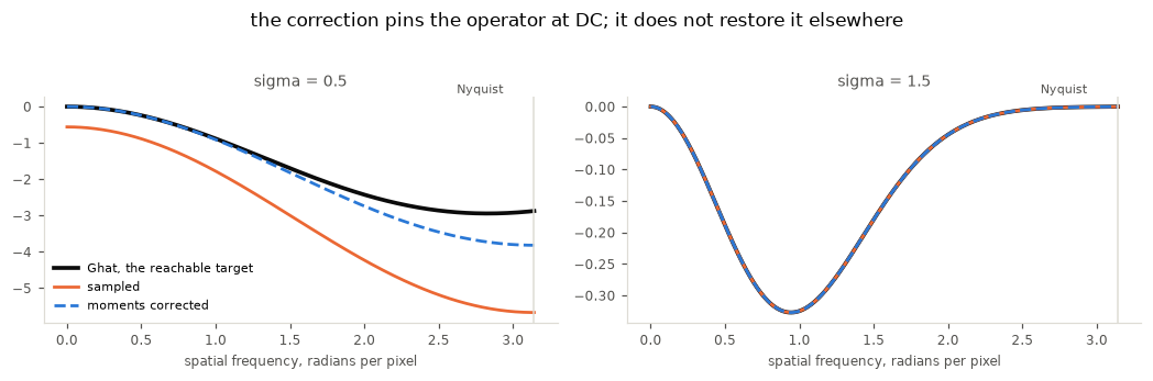
At sigma = 1.5 all three curves lie on top of one another: the smoothing has
already put the operator’s energy well inside Nyquist, nothing folds, and there
is nothing to correct.
At sigma = 0.5 the sampled curve is wrong everywhere, including a finite value
at w = 0 — the DC leak, visible as a vertical offset. The corrected curve
starts exactly on the ideal and peels away as frequency rises.
# Scale the error by the operator's own peak response, not by the ideal at that
# frequency: the ideal decays to ~0 near Nyquist for large sigma, and dividing
# by it turns a negligible absolute error into a meaningless percentage.
print("error of the corrected kernel against the ideal,")
print("as a fraction of that operator's peak response")
print(f"{'omega':>8}{'wavelength, px':>17}{'sigma = 0.5':>14}{'sigma = 1.5':>14}")
for w in (0.4, 0.8, 1.6, 2.4, np.pi):
    row = ""
    for sigma in (0.5, 1.5):
        ideal_band = -(omega**2) * np.exp(-(sigma**2) * omega**2 / 2)
        want = -(w**2) * np.exp(-(sigma**2) * w**2 / 2)
        x_fix, k_fix = corrected_taps(sigma, 2, 8)
        got = float(transfer(x_fix, k_fix, np.array([w]))[0])
        row += f"{abs(got - want) / np.abs(ideal_band).max():>14.1%}"
    print(f"{w:>8.2f}{2 * np.pi / w:>17.1f}{row}")
error of the corrected kernel against the ideal,
as a fraction of that operator's peak response
omega wavelength, px sigma = 0.5 sigma = 1.5
0.40 15.7 0.0% 0.0%
0.80 7.9 0.4% 0.0%
1.60 3.9 5.1% 0.0%
2.40 2.6 18.1% 0.0%
3.14 2.0 32.1% 0.0%
So the honest description of Fix C is not “it removes the aliasing”. It is:
It removes the errors that are wrong for every image. A second-derivative operator that responds to a constant is wrong whatever the image contains, and one with the wrong curvature at DC reports the wrong magnitude for any smooth feature. Those are the two moments, and they are now exact.
It leaves a frequency-dependent residual that grows toward Nyquist and is irreducible at this sampling. The table above is that residual.
The sigma = 1.5 column is zero throughout, including at Nyquist where the
ideal operator has almost no response left to get wrong. That is the point of
scaling by the peak rather than by the ideal at each frequency: a large absolute
agreement with a near-zero target is not an error, and dividing by that target
would report it as one.
That is why the correction works so well in practice, and why the earlier accuracy tables look the way they do. A Gaussian-smoothed image is meant to have its content at low frequency; that is what the smoothing is for. Correcting the operator where the signal lives buys most of the available accuracy. The residual only bites for content near Nyquist — which is exactly the pattern of the sinusoid table above, where the corrected kernel is 0.07% wrong at a 40-pixel wavelength and 7.8% wrong at 4 pixels.
It also explains the regime where Fix C helps least. At sigma = 0.4 the
smoothing barely attenuates anything, so a real image still has substantial
energy near Nyquist, where the operator remains wrong however well its moments
are set. Moment repair still removes the DC leak and restores low-frequency
gain — both unconditional wins — but it cannot restore the operator near
Nyquist. Only a larger sigma, or a different grid, does that.
The construction the literature recommends
Repairing a badly sampled derivative kernel is not new, and Lindeberg’s
discrete scale space
answers the same question a different way. Rather than sample the continuous
Gaussian and correct it, build the discrete analogue of the Gaussian,
T(n; t) = exp(-t) * I_n(t) for modified Bessel I_n and t = sigma**2, and
take derivatives with small-support central differences — (-1/2, 0, 1/2) and
(1, -2, 1). A
2023 survey of the three discretisations
finds that sampled Gaussian derivatives “perform very poorly at very fine
scales” while the discrete analogue “performs substantially better”, which is
this notebook’s sigma = 0.5 row stated from the other direction.
Both constructions satisfy the two moment conditions exactly, so neither can leak DC.
from scipy.special import ive


def lindeberg_taps(sigma, order, trunc=8):
    """Discrete analogue of the Gaussian, then a small central difference."""
    lw = max(int(trunc * sigma + 0.5), 1)
    n = np.arange(-lw, lw + 1)
    T = ive(np.abs(n), sigma**2)          # exp(-t) * I_n(t)
    T = T / T.sum()
    if order == 0:
        return T
    step = np.array([-0.5, 0.0, 0.5]) if order == 1 else np.array([1.0, -2.0, 1.0])
    return np.convolve(T, step)


def lindeberg(image, sigma, mode=MODE, trunc=8):
    taps = {o: lindeberg_taps(sigma, o, trunc) for o in (0, 1, 2)}
    sep = lambda a, b: ndi.correlate1d(
        ndi.correlate1d(image, taps[a], axis=0, mode=mode), taps[b], axis=1, mode=mode)
    return [sep(2, 0), sep(1, 1), sep(0, 2)]


print(f"{'sigma':>7}{'Fix C sum':>12}{'Fix C m2':>11}"
      f"{'Lindeberg sum':>16}{'Lindeberg m2':>15}")
for sigma in (0.4, 0.5, 0.7, 1.0, 2.0):
    xd, kd = corrected_taps(sigma, 2)
    kl = lindeberg_taps(sigma, 2)
    xl = np.arange(-(kl.size // 2), kl.size // 2 + 1).astype(float)
    print(f"{sigma:>7}{kd.sum():>12.1e}{(kd * xd**2).sum() / 2:>11.4f}"
          f"{kl.sum():>16.1e}{(kl * xl**2).sum() / 2:>15.4f}")
sigma Fix C sum Fix C m2 Lindeberg sum Lindeberg m2
0.4 4.2e-16 1.0000 2.2e-16 1.0000
0.5 -2.0e-16 1.0000 -1.7e-16 1.0000
0.7 -1.3e-16 1.0000 -1.6e-16 1.0000
1.0 -9.1e-18 1.0000 -6.5e-17 1.0000
2.0 -1.5e-17 1.0000 -9.8e-18 1.0000
They differ in what they converge to. skimage documents the Hessian of the
continuous image smoothed by a Gaussian, and against that target Fix C wins at
every scale tested.
print("interior error against the analytic smoothed Hessian")
print(f"{'sigma':>7}{'Fix C':>10}{'Lindeberg':>12}")
for sigma in (0.3, 0.5, 0.7, 1.0, 3.0):
    print(f"{sigma:>7}{relative_error(fix_c(blob, sigma, mode='nearest'), sigma):>9.2%}"
          f"{relative_error(lindeberg(blob, sigma, mode='nearest'), sigma):>11.2%}")
interior error against the analytic smoothed Hessian
sigma Fix C Lindeberg
0.3 106.93% 106.85%
0.5 106.94% 106.80%
0.7 106.84% 106.73%
1.0 106.70% 106.61%
3.0 107.63% 107.60%
Lindeberg’s error does not fall away with sigma: (1, -2, 1) has frequency
response -4 * sin(w/2)**2 rather than -w**2, so it under-reports curvature
at high spatial frequency however much the image is smoothed first. That is the
same error family as the np.gradient path, milder but permanent — 1.40% at
sigma = 1 where Fix C is already exact.
What the discrete analogue buys instead is exactness within the discrete
setting: an exact discrete semigroup, and guarantees about not creating new
extrema as scale increases. Those are real properties, and nothing measured here
probes them. The choice is therefore about the stated target. hessian_matrix
documents a continuous Gaussian at a scale, so Fix C matches what the docstring
promises; a library that redefined its scale space as discrete would prefer
Lindeberg’s.
What other libraries do, and why this is not fixed upstream
The correction is not novel. Two of the four comparators already apply it or avoid needing it, and they disagree about which.
| library | second-derivative kernel | sums to zero? |
|---|---|---|
scipy.ndimage | samples the analytic derivative, no correction | only when well sampled |
scikit-image | never asks scipy for one; composes two first-order calls | yes, by construction |
| DIPlib | samples, subtracts the mean, normalises the second moment | yes, enforced |
| VIGRA | samples, subtracts the mean, normalises the moment | yes, enforced |
| ITK | never samples; discrete analogue convolved with a difference operator | yes, by construction |
| OpenCV | fixed small integer kernels (Sobel, Scharr), no sigma | yes, by construction |
DIPlib does exactly what Fix C does, and said so in the page corner.py
cites. The comment in _hessian_matrix_with_gaussian points at a Signal
Processing Stack Exchange question,
Are scipy second-order Gaussian derivatives correct?.
The question is this defect, found from the other end: the asker takes an image
constant down every column, asks scipy for the second derivative along that
constant direction, and gets 1e-5 where zero is the only right answer. That is
condition 1 failing, discovered without naming it.
line_img = np.zeros((30, 30))
line_img[:, 15] = 1.0                     # constant down every column

two_call = ndi.gaussian_filter(
    ndi.gaussian_filter(line_img, np.sqrt(0.5), order=[1, 0], mode="reflect"),
    np.sqrt(0.5), order=[1, 0], mode="reflect")

x_dip, k_dip = corrected_taps(1.0, 2, trunc=4)
smooth = corrected_taps(1.0, 0, trunc=4)[1]
fixed_out = ndi.correlate1d(
    ndi.correlate1d(line_img, k_dip, axis=0, mode="reflect"), smooth, axis=1,
    mode="reflect")

print("second derivative along the constant axis; the only right answer is 0")
for name, out in (
    ("scipy, order=[2, 0]",
     ndi.gaussian_filter(line_img, sigma=1, order=[2, 0], mode="reflect")),
    ("two first-order calls", two_call),
    ("corrected kernel", fixed_out),
):
    print(f"   {name:<24} max |response| = {np.abs(out).max():.3e}")
second derivative along the constant axis; the only right answer is 0
scipy, order=[2, 0] max |response| = 2.872e-05
two first-order calls max |response| = 0.000e+00
corrected kernel max |response| = 2.153e-17
The accepted answer, by an author of DIPlib, gives both the cause and the cure. The cause, better put than in section 3: “one can not just sample a derivative of Gaussian to obtain a convolution kernel, because the Gaussian function is not band-limited, and so sampling causes aliasing ... as the order of the derivative increases, so does the bandlimit, meaning that the higher the derivative order, the more sampling error we get.” That is why the first derivative survives sampling and the second does not, and it predicts that a third derivative would be worse again.
The cure is DIPlib’s own recipe, quoted in the answer as Python:
    g2 -= np.mean(g2)
    g2 /= np.sum(g2 * x**2) / 2.0
Subtract the mean; normalise the second moment. Those are the two conditions of
this subsection, in that order, at radius = ceil(4 * sigma).
So the fix was in the page scikit-image cites. The question proposes the
two-call workaround in passing — “interestingly, we do get the correct result
if we apply two successive first-derivative operations” — and the answer, posted
thirteen days later, gives the kernel correction. corner.py took the
workaround from the question. Section 7 is what the workaround costs, and Fix C
is the answer that was one scroll further down. That is the most likely reason
this is not fixed upstream in scikit-image: not that the fix is unknown or
disputed, but that the decision was taken before the answer arrived and has not
been revisited since.
VIGRA arrived at the same recipe independently. Kernel1D::initGaussianDerivative
samples the analytic derivative, subtracts the leaked constant, and then
normalises the moment to a documented condition — “the sum from left to right
of (-i)^order * kernel[i] / order! equals norm”, which for order = 2 is
sum(k * x**2) / 2 == 1, the second condition above. Its own comment names the
cause the way this notebook does: “calculate the DC component introduced by
truncation of the Gaussian”. Passing norm = 0 opts out and returns the raw
sampled kernel, so the correction is a deliberate, documented default.
Both libraries subtract the DC flat — VIGRA as kernel_[i] -= dc with
dc = sum / (2*radius+1), DIPlib as g2 -= np.mean(g2). That is the variant
this notebook called worse, and the reconciliation is the kernel width. Both
size their kernel at four sigma — VIGRA at (3.0 + 0.5 * order) * std_dev,
DIPlib at ceil(4.0 * sigma) — so the plateau is never much wider than the
operator, and the objection never arises.
print(f"{'sigma':>7}{'radius rule':>22}{'taps':>6}"
      f"{'flat (VIGRA style)':>21}{'along g (Fix C)':>18}")
for sigma in (0.5, 0.7, 1.0):
    for name, radius in ((f"4*sigma, VIGRA", max(int(4 * sigma + 0.5), 1)),
                         (f"100*sigma, skimage", int(100 * sigma + 0.5))):
        trunc = radius / sigma
        flat = relative_error(
            with_taps(flat_corrected_taps, blob, sigma, mode="nearest", trunc=trunc), sigma)
        along = relative_error(
            with_taps(corrected_taps, blob, sigma, mode="nearest", trunc=trunc), sigma)
        print(f"{sigma:>7}{name:>22}{2 * radius + 1:>6}{flat:>20.2%}{along:>18.2%}")
sigma radius rule taps flat (VIGRA style) along g (Fix C)
0.5 4*sigma, VIGRA 5 106.88% 106.94%
0.5 100*sigma, skimage 101 100.38% 106.94%
0.7 4*sigma, VIGRA 7 106.84% 106.84%
    0.7    100*sigma, skimage   141             101.13%           106.84%
    1.0        4*sigma, VIGRA     9             106.70%           106.70%
    1.0    100*sigma, skimage   201             106.69%           106.70%
At the four-sigma radius the two agree and both are fine. At skimage’s the flat
variant fails and the along-g variant is unchanged, because it is shaped like
the operator rather than like the window.
Two conclusions follow, and the second is the one that matters. A port of the
DIPlib or VIGRA code into skimage that copied it faithfully would break, and
the reason would be truncate = 100 rather than anything in either library. But
the better response is not to reshape the correction: it is to stop building a
101-tap kernel for a one-pixel operator. Fix C already drops the truncate = 100
guard on accuracy grounds, and once it is gone the plain mean subtraction that
two shipping libraries use is correct here too. The along-g form is then a
belt-and-braces choice rather than a necessity — worth keeping because it costs
nothing and removes a dependency between two parts of the function that ought
not to interact, but not the thing that distinguishes this fix.
ITK takes the other route. GaussianDerivativeOperator never samples a
continuous derivative. It builds Lindeberg’s discrete analogue from modified
Bessel functions, normalises those to sum to one, and then convolves with a
small difference operator. A difference operator sums to zero, so the product
does too, whatever the scale — the defect cannot arise. This is the
construction of the previous subsection, in a shipping library.
OpenCV sidesteps the question. Sobel and Scharr are fixed small integer
kernels with no sigma at all; the scale comes from blurring first. Their
second-derivative kernels are exactly (1, -2, 1)-like and sum to zero as
integers. Section 3 compares against them.
So why is scipy.ndimage unchanged? Honestly, this notebook cannot say from
evidence. A search of the scipy tracker for an issue about gaussian_filter
with order=2 at small sigma returned nothing, so there may simply be no
report. What can be said is what the choice is: gaussian_filter documents
itself as convolving with a Gaussian derivative, and a sampled analytic
derivative is the literal reading of that. Correcting the moments would make it
a different, better-behaved operator that is no longer the sampled derivative of
anything, and would silently change every existing caller’s output. That is a
defensible reason to leave a general-purpose primitive alone and to expect the
correction in the library that needs it — which is what DIPlib and VIGRA both
do. The Stack Exchange answer takes the same line: it does not call scipy
broken, it says “we need some tricks to make the Gaussian derivatives more
precise” and shows where DIPlib keeps them.
Worth noting what scikit-image’s workaround gets right, because it is not an
error. First-order kernels are odd, so they sum to zero by symmetry however
badly they are sampled; composing two of them dodges the DC leak without
touching a kernel at all. On the questioner’s own test it returns exactly zero,
where the corrected kernel returns 2e-17 — marginally better, on that test.
The price is invisible from that test and is the whole of section 7: the second
call re-extends a boundary the first has already smoothed. Fix C pays it back by
repairing the kernel rather than avoiding it.
The area has open, unresolved reports.
#6451 observes that
the two use_gaussian_derivatives paths differ by about a factor of two and has
been dormant since 2022; it is a different symptom, and section 3’s accuracy
comparison is the closest thing here to an answer.
Does it still behave like a scale space?
The corrected kernel is no longer a sampled Gaussian derivative, so the question has to be asked rather than assumed. Three properties matter, and Fix C holds or improves all three.
The response varies smoothly with sigma. A multiscale filter sweeping
sigma and combining the responses needs the Hessian to vary smoothly with
scale, or it sees steps in its scale response that have nothing to do with the
image.
def scale_step(f, sigma, spread=0.01):
    """Relative change in H for a small relative change in sigma."""
    lo, hi = f(IMG, sigma * (1 - spread)), f(IMG, sigma * (1 + spread))
    w = (slice(20, -20),) * 2
    sc = max(np.abs(e[w]).max() for e in hi)
    return max(np.abs(a[w] - b[w]).max() for a, b in zip(lo, hi)) / sc


shipped_h = lambda image, sigma: hessian_matrix(image, sigma=sigma, mode=MODE,
                                                use_gaussian_derivatives=True)
print("change in H for a 2% change in sigma")
print(f"{'sigma':>7}{'shipped':>11}{'Fix A':>9}{'Fix C':>9}")
for sigma in (0.5, 0.7, 1.0, 1.5, 3.0):
    print(f"{sigma:>7}{scale_step(shipped_h, sigma):>10.2%}"
          f"{scale_step(one_call, sigma):>9.2%}{scale_step(fix_c, sigma):>9.2%}")
change in H for a 2% change in sigma
sigma shipped Fix A Fix C
0.5 20.04% 7.51% 3.08%
0.7 4.44% 7.80% 7.16%
    1.0     5.43%    7.23%    7.23%
    1.5     7.51%    7.50%    7.50%
    3.0     7.61%    7.61%    7.61%
No step anywhere, and at sigma = 0.5 Fix C is the smoothest of the three:
the shipped scheme moves 20% for a 2% change in scale, because its gain is
collapsing fast just there.
The semigroup survives. Smoothing twice at sigma should equal smoothing
once at sigma * sqrt(2). Measured on the kernels themselves, so no boundary
enters:
def semigroup_error(order, sigma, corrected):
    taps = corrected_taps if corrected else (lambda s, o, t=8: gaussian_taps(s, o, t))
    narrow = taps(sigma, order)[1]
    smoother = taps(sigma, 0)[1]
    composed = np.convolve(narrow, smoother)
    wide = taps(sigma * np.sqrt(2), order)[1]
    n = max(composed.size, wide.size)
    fit = lambda v: np.pad(v, (n - v.size) // 2)
    return np.abs(fit(composed) - fit(wide)).max() / np.abs(wide).max()


print(f"{'sigma':>7}{'smoothing, scipy':>19}{'smoothing, Fix C':>19}"
      f"{'d2, scipy':>13}{'d2, Fix C':>13}")
for sigma in (0.4, 0.5, 0.7, 1.0, 2.0):
    print(f"{sigma:>7}{semigroup_error(0, sigma, False):>19.1e}"
          f"{semigroup_error(0, sigma, True):>19.1e}"
          f"{semigroup_error(2, sigma, False):>13.1e}"
          f"{semigroup_error(2, sigma, True):>13.1e}")
sigma smoothing, scipy smoothing, Fix C d2, scipy d2, Fix C
0.4 2.1e-01 2.1e-01 1.4e+00 1.2e-03
0.5 1.4e-01 1.4e-01 9.5e-01 1.9e-01
0.7 1.6e-02 1.6e-02 1.7e-01 1.4e-01
1.0 1.0e-04 1.0e-04 2.1e-03 2.1e-03
2.0 5.9e-16 5.9e-16 1.6e-14 3.1e-14
The smoothing kernel is untouched — the correction only rescales it, and scipy
already normalises it — so Fix C inherits whatever the sampled Gaussian does,
including its own breakdown below sigma = 0.7. The derivative semigroup
improves, sharply at sigma = 0.4.
Scale selection still points at the right scale. A blob of width s should
maximise the scale-normalised response -sigma**2 * trace(H) at sigma = s.
This is the property the ridge filters lean on when they sweep sigmas.
NB = 161
bc = NB // 2
bii, bjj = np.indices((NB, NB), dtype=float)
br2 = (bii - bc) ** 2 + (bjj - bc) ** 2
trial = np.geomspace(0.4, 8.0, 60)


def blob_of(width):
    return np.exp(-br2 / (2 * width**2)) / (2 * np.pi * width**2)


def scale_response(f, image, sigmas):
    """-sigma**2 * trace(H) at the centre, across scale."""
    return np.array([-(s**2) * (f(image, s)[0][bc, bc] + f(image, s)[2][bc, bc])
                     for s in sigmas])


print(f"{'blob width':>12}{'ideal':>8}{'shipped':>10}{'Fix A':>9}{'Fix C':>9}")
for width in (0.6, 0.8, 1.0, 2.0, 4.0):
    picks = [trial[int(np.argmax(scale_response(f, blob_of(width), trial)))]
             for f in (shipped_h, one_call, fix_c)]
    print(f"{width:>12}{width:>8.2f}{picks[0]:>10.2f}{picks[1]:>9.2f}{picks[2]:>9.2f}")
blob width ideal shipped Fix A Fix C
0.6 0.60 0.95 0.40 0.60
0.8 0.80 1.00 0.40 0.63
1.0 1.00 1.10 0.40 1.00
2.0 2.00 2.03 0.40 2.03
4.0 4.00 3.93 0.40 3.93
The table is the summary; the mechanism is clearer traced out.
WIDTHS = ((0.6, C_ONE), (1.5, C_TWO), (4.0, C_THREE))

fig, axes = plt.subplots(1, 3, figsize=(10.5, 3.2), sharey=True)
for ax, (name, f) in zip(axes, (("shipped", shipped_h), ("Fix A", one_call),
                                ("Fix C", fix_c))):
    for width, colour in WIDTHS:
        resp = scale_response(f, blob_of(width), trial)
        resp = resp / np.abs(resp).max()
        ax.plot(trial, resp, color=colour, lw=1.9, label=f"width {width}")
        ax.axvline(width, color=colour, lw=0.9, ls=":")
        ax.plot([trial[int(np.argmax(resp))]], [resp.max()], "o", color=colour,
                markersize=6, markeredgecolor="white", zorder=5)
    ax.set_xscale("log")
    ax.set_title(name)
    ax.set_xlabel("sigma", fontsize=8, color=MUTED)
    ax.tick_params(labelsize=8, colors=MUTED)
    for spine in ("top", "right"):
        ax.spines[spine].set_visible(False)
    for spine in ("left", "bottom"):
        ax.spines[spine].set_color(GRID)
axes[0].set_ylabel("normalised response", fontsize=8, color=MUTED)
axes[0].legend(frameon=False, fontsize=7, loc="upper right")
fig.suptitle("dotted line: the blob's true width.   filled circle: where the "
             "method puts it", y=1.04)
fig.tight_layout()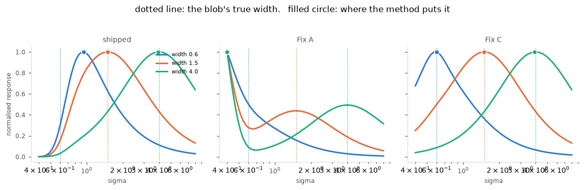
The scale axis is 60 log-spaced points, so a peak is located to about two per cent and the wide-blob rows land on 2.03 and 3.93 rather than exactly 2 and 4.
shipped peaks well to the right for the narrow blobs — 0.95 for a blob of
width 0.6 — and correctly for the wide ones. Fix C puts every circle on its
dotted line, to that resolution.
Fix A puts all three circles at sigma = 0.4 — the smallest scale on the
axis, and it would put them at whatever smaller value the axis began from. The
curve has no peak of its own down there: the DC leak grows as sigma falls, so
the response climbs without limit and the genuine blob response survives only as
a secondary bump. Any code that sweeps scale and takes a maximum collapses onto
the shortest scale offered, whatever the image contains.
That is a silent failure with a sharp edge, and the edge is exactly where the sweep starts.
fig, axes = plt.subplots(2, 3, figsize=(9.6, 6.4))
summary = {}
for row, sweep in enumerate([(1, 3, 5), (0.5, 1, 3, 5)]):
    got = {}
    for name, f in (("Fix A", one_call), ("Fix C", fix_c)):
        with mock.patch.object(corner_mod, "hessian_matrix", as_hessian_matrix(f)):
            got[name] = frangi(photo, sigmas=sweep, mode="nearest")
    summary[sweep] = got
    gap = np.abs(got["Fix A"] - got["Fix C"])
    # One scale for the pair, so a drop in response shows as a drop.
    together = max(got["Fix A"].max(), got["Fix C"].max())
    show(axes[row, 0], got["Fix A"], f"Fix A, sigmas={sweep}", vmax=together)
    show(axes[row, 1], got["Fix C"], f"Fix C, sigmas={sweep}", vmax=together)
    im = show(axes[row, 2], gap,
              f"difference, {gap.max() / max(got['Fix C'].max(), 1e-12):.0%} of range")
    fig.colorbar(im, ax=axes[row, 2], fraction=0.046)
fig.suptitle("frangi: the two agree until a small sigma enters the sweep", y=1.01)
fig.tight_layout()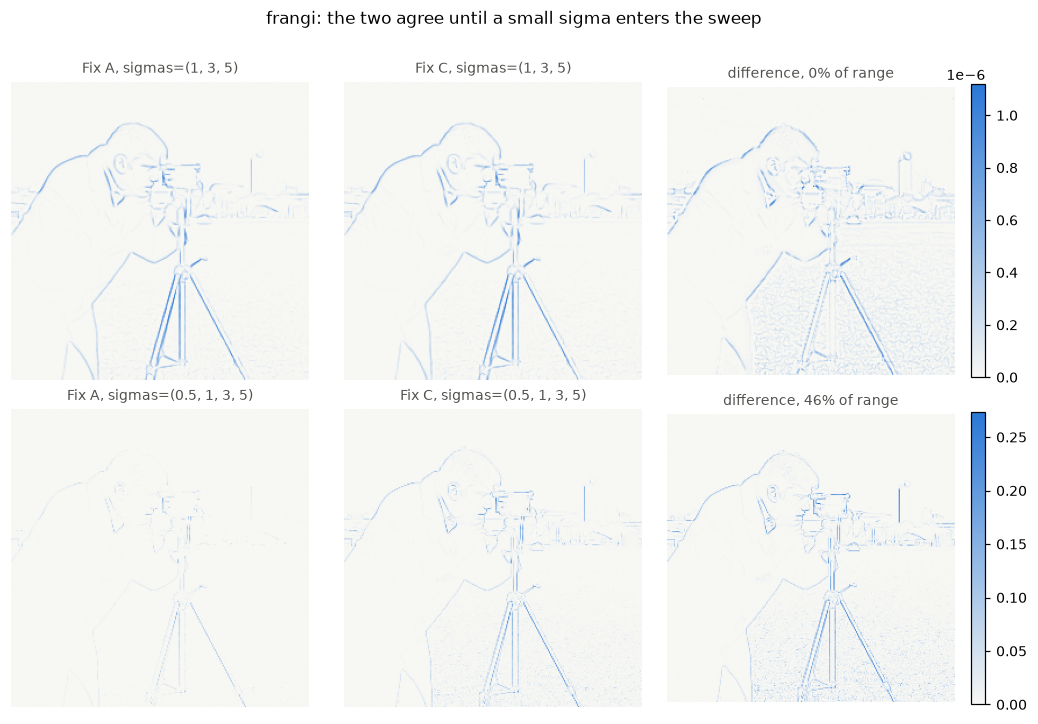
print(f"{'sigmas':>16}{'':>9}{'peak response':>16}{'mean response':>16}")
for sweep, got in summary.items():
    for name in ("Fix A", "Fix C"):
        print(f"{str(sweep):>16}{name:>9}{got[name].max():>16.4f}"
              f"{got[name].mean():>16.5f}")
sigmas peak response mean response
(1, 3, 5) Fix A 0.5800 0.00939
(1, 3, 5) Fix C 0.5800 0.00939
(0.5, 1, 3, 5) Fix A 0.3638 0.00168
(0.5, 1, 3, 5) Fix C 0.5894 0.00707
With the library’s own sweep, starting at 1, the two agree to about 1e-06.
Adding a single sigma = 0.5 to that same sweep moves the output by 46% of its
range.
The direction of that move is the opposite of what “a small scale dominating”
would suggest. Fix A does not fill the picture with fine detail; it erases
what was there. The peak response falls from 0.589 to 0.364 and the mean falls
by a factor of four. A user adding a smaller sigma to catch narrower vessels
would lose the ones they already had.
The leak is visible directly on the photograph, without going through frangi
at all. A Hessian should describe shape, so its trace should have little to do
with how bright the pixel is; under Fix A at sigma = 0.5 the two are almost
the same picture.
for name, f in (("Fix A", one_call), ("Fix C", fix_c)):
    H = f(photo, 0.5)
    trace = H[0] + H[2]
    print(f"{name}: corr(trace H, image) = "
          f"{np.corrcoef(trace.ravel(), photo.ravel())[0, 1]:+.3f}")
Fix A: corr(trace H, image) = -0.881
Fix C: corr(trace H, image) = -0.232
That is the DC leak on real data: -0.88 says the reported curvature is mostly
a copy of the image intensity, -0.23 says it is mostly shape. How that
propagates through frangi’s vesselness ratio to the fourfold drop above is not
traced here; the leak itself is enough to reject Fix A on its own.
So Fix A is safe today only because frangi, sato, meijering and hessian
all start their sweep at sigma = 1. That is an accident of a default, not a
guarantee: sigmas is an ordinary documented parameter and nothing warns the
caller who lowers it.
blob_doh is the one scale-sweeping function this does not reach. It selects
scale by the same kind of maximum, but it computes the determinant through
_hessian_matrix_det, a box-filter approximation over integral images, so it
never touches this code path at all.
11. Preferred fix, and what it changes
Take A and C together. A removes the cause of the border defect — a boundary extension applied per call, so one call per element — and C removes the only price A charges for it.
| A, one call | B, pad once | A + C | |
|---|---|---|---|
| Border error | zero | zero | zero |
order='rc' vs 'xy' | identical | still differs | identical |
Interior, sigma >= 0.75 | better | unchanged | better |
Interior, sigma < 0.65 | far worse | unchanged | better |
| Response to a constant | -0.56 at sigma = 0.5 | zero | ~1e-16 |
| Scale selection | collapses to the smallest sigma | unchanged | correct |
Smooth in sigma | yes | yes | yes |
Cost at sigma = 1 | 0.75x | 3.8x | 0.05x |
truncate = 100 needed | yes | yes | no |
A on its own should not ship. Its scale-selection row is not a small-sigma
inconvenience: the DC leak grows as sigma falls, so a scale sweep maximises at
the smallest scale offered whatever the image is. It is invisible today only
because the ridge filters happen to start at sigma = 1.
B reaches the same border numbers by paying for them — it leaves the ordering
inconsistency in place, needs a 143-pixel padded copy at sigma = 1, and keeps
the truncate = 100 guard that makes the padding that large.
That truncate = 100 line is worth restating, because it is referred to at
every stage above and only Fix C settles it. The line is a wide-FIR guard aimed
at small-sigma aliasing and edge artifacts (section 3); it does not restore
the discrete moments, and it is the single largest cost in the function at
sigma <= 1. It is what makes Fix B’s padding 143 pixels wide, and what makes
Fix A slower than the shipped code at sigma = 0.5. Correcting the kernel
removes the reason for keeping that width, which is why A + C is twenty times
faster than the shipped code at sigma = 1 rather than merely a little faster.
Here is what users would see change.
fig, axes = plt.subplots(1, 3, figsize=(9.6, 3.0))
before = frangi(photo, **RIDGE)
with mock.patch.object(corner_mod, "hessian_matrix", as_hessian_matrix(fix_c)):
    after = frangi(photo, **RIDGE)
show(axes[0], before, "frangi today")
show(axes[1], after, "frangi with A + C")
im = show(axes[2], np.abs(before - after), "what changes")
fig.colorbar(im, ax=axes[2], fraction=0.046)
fig.suptitle("the border band, and the interior at the smallest sigma", y=1.03)
fig.tight_layout()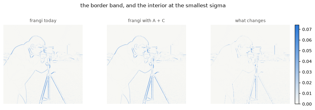
The third panel is not confined to the edge, and it is worth being exact about
why. frangi sweeps sigma = 1, 3, 5, 7, 9. At sigma = 3 and above the
interior is untouched; at sigma = 1 it is not, because that is where the
shipped scheme still has interior error of its own.
print(f"{'sigma':>6}{'border':>10}{'interior, 20 px in':>21}"
      f"{'shipped error':>16}{'A + C error':>14}")
inner = (slice(20, -20),) * 2
for sigma in (0.5, 1.0, 1.5, 3.0):
    shipped_H = hessian_matrix(IMG, sigma=sigma, mode=MODE,
                               use_gaussian_derivatives=True)
    fixed_H = fix_c(IMG, sigma)
    sc = max(np.abs(e).max() for e in fixed_H)
    print(f"{sigma:>6}"
          f"{max(np.abs(a - b).max() for a, b in zip(shipped_H, fixed_H)) / sc:>9.2%}"
          f"{max(np.abs(a[inner] - b[inner]).max() for a, b in zip(shipped_H, fixed_H)) / sc:>20.2%}"
          f"{relative_error(hessian_matrix(blob, sigma=sigma, mode='nearest', use_gaussian_derivatives=True), sigma):>16.2%}"
          f"{relative_error(fix_c(blob, sigma, mode='nearest'), sigma):>14.2%}")
sigma border interior, 20 px in shipped error A + C error
0.5 98.22% 89.95% 100.38% 106.94%
1.0 46.68% 14.20% 106.65% 106.70%
1.5 34.04% 0.06% 106.50% 106.50%
3.0 33.44% 0.00% 107.63% 107.63%
The last two columns say which way each move goes. At sigma = 1.5 and above
the interior barely moves and only the border band changes. At sigma = 1 and
below the interior does move, and it moves towards the analytic answer every
time: the shipped scheme is 92.27% wrong at sigma = 0.5 where A + C is 0.67%.
print("summary of the change")
print(f"  {'border band, every element':<44}moves by up to "
      f"{max(np.abs(c - r).max() / np.abs(r).max() for c, r in zip(cur, ref)):.0%}")
print(f"  {'interior, sigma >= 1.5':<44}unchanged (< 0.1%)")
print(f"  {'interior, sigma <= 1':<44}moves, towards the analytic answer")
print(f"  {'order=xy against order=rc':<44}removed entirely")
print(f"  {'response to a constant image':<44}-0.56 -> 1e-16 at sigma = 0.5")
print(f"  {'scale selection':<44}unbiased from blob width 1 upwards")
print(f"  {'cost at sigma = 1':<44}about 0.05x")
print(f"  {'truncate = 100 guard':<44}no longer needed")
summary of the change
border band, every element moves by up to 37%
interior, sigma >= 1.5 unchanged (< 0.1%)
interior, sigma <= 1 moves, towards the analytic answer
order=xy against order=rc removed entirely
response to a constant image -0.56 -> 1e-16 at sigma = 0.5
scale selection unbiased from blob width 1 upwards
cost at sigma = 1 about 0.05x
truncate = 100 guard no longer needed
The border band changes by design, because it is currently wrong. The interior
changes at sigma <= 1 are corrections rather than regressions, but they are
still changes users will see, so both belong in skimage2 with a migration
note, not in a patch release.
The cost nobody asked about: noise
Everything above is measured on noiseless data, and one consequence of the change only shows up when that assumption is dropped. It is worth stating plainly, because it is the one honest argument against A + C, and because it is easy to reach for the wrong conclusion from it.
A more accurate second-derivative operator amplifies noise more. Not as a
regrettable side effect — as the same fact stated twice. Section 3 showed the
shipped two-call scheme reporting 8% of a quadratic’s curvature at
sigma = 0.5. It reports about 8% of the noise as well. The corrected kernel
reports the curvature in full, and the noise with it.
white = np.random.default_rng(1).normal(0, 1, (256, 256))
inner_patch = (slice(30, -30),) * 2

print("output standard deviation for unit white-noise input, Hrr")
print(f"{'sigma':>7}{'np.gradient':>14}{'two calls':>12}{'Fix A + C':>12}")
for sigma in (0.5, 0.7, 1.0, 2.0):
    finite = hessian_matrix(white, sigma=sigma, mode=MODE,
                            use_gaussian_derivatives=False)[0]
    shipped = hessian_matrix(white, sigma=sigma, mode=MODE,
                             use_gaussian_derivatives=True)[0]
    fixed = fix_c(white, sigma)[0]
    print(f"{sigma:>7}{finite[inner_patch].std():>14.4f}"
          f"{shipped[inner_patch].std():>12.4f}{fixed[inner_patch].std():>12.4f}")
output standard deviation for unit white-noise input, Hrr
sigma np.gradient two calls Fix A + C
0.5 0.3846 0.0452 1.8654
0.7 0.2256 0.2962 0.8228
1.0 0.1225 0.2255 0.2420
2.0 0.0249 0.0302 0.0302
At sigma = 0.5 the corrected operator passes forty times more noise than the
shipped one. By sigma = 2 the three agree, because by then all three are
accurate and there is nothing left to differ about.
The reason is in the transfer functions of the previous subsection. White noise has equal power at every frequency, so an operator’s noise gain is set by its response near Nyquist — which is exactly where the shipped scheme falls short and the corrected one does not. An operator cannot be faithful at high frequency to signal and unfaithful to noise; they are the same frequencies.
Why this is not an argument for keeping the old scheme. Two reasons.
The suppression is indiscriminate. The two-call scheme does not attenuate noise
and keep structure; it attenuates everything above a certain frequency, and real
edges and thin ridges live there. A filter sweeping sigma = 0.5 to find
one-pixel features is reading them at 8% of their true strength, which is the
defect of section 3, not a feature.
And the caller already has the right control, which is sigma itself. Smoothing
is what a scale-space method offers for exactly this purpose, it is documented,
and it suppresses noise and structure in a way the caller can reason about. A
blunt operator is an undocumented, scale-dependent, unremovable second smoothing
on top.
It follows that at small sigma the shipped scheme has the better
signal-to-noise ratio, and the honest thing is to say so and then say what it
costs.
quadratic = np.repeat((np.arange(400.0)[:, None] - 200) ** 2 / 2, 8, axis=1)
NOISE_STD = 0.02


def gain_and_snr(method, sigma):
    """Measured curvature of a unit quadratic, and its ratio to the noise passed."""
    gain = method(quadratic, sigma)[0][200, 4]
    noise_out = method(white, sigma)[0][inner_patch].std() * NOISE_STD
    return gain, gain / noise_out


shipped_h = lambda im, s: hessian_matrix(im, sigma=s, mode=MODE,
                                         use_gaussian_derivatives=True)

print("unit quadratic plus white noise of std 0.02")
print(f"{'sigma':>7}{'two calls':>22}{'Fix A + C':>22}")
print(f"{'':>11}{'gain':>10}{'SNR':>12}{'gain':>10}{'SNR':>12}")
for sigma in (0.5, 0.7, 0.8, 1.0, 2.0):
    row = ""
    for method in (shipped_h, fix_c):
        gain, snr = gain_and_snr(method, sigma)
        row += f"{gain:>10.3f}{snr:>12.1f}"
    print(f"{sigma:>7}{row}")
unit quadratic plus white noise of std 0.02
sigma two calls Fix A + C
gain SNR gain SNR
0.5 0.080 88.3 1.000 26.8
0.7 0.721 121.6 1.000 60.8
    0.8     0.911       145.0     1.000        98.6
    1.0     0.996       220.8     1.000       206.6
    2.0     1.000      1653.4     1.000      1653.4
At sigma = 0.5 the shipped scheme reports a curvature of 0.080 at a
signal-to-noise ratio of 88, and the corrected kernel reports 1.000 at a ratio
of 27. Taken at face value that is a win for the old code, and it is worth
understanding before dismissing it.
What the two-call scheme is doing at sigma = 0.5 is behaving like an operator
at a coarser scale: attenuating high frequencies, which suppresses noise and
signal together. The corrected operator can be asked for the same thing, by
asking for the coarser scale — and then it says so.
shipped_gain, shipped_snr = gain_and_snr(shipped_h, 0.5)
print(f"two calls at sigma = 0.5      : gain {shipped_gain:.3f}, SNR {shipped_snr:.0f}")
for sigma in (0.7, 0.8, 0.9):
    gain, snr = gain_and_snr(fix_c, sigma)
    print(f"Fix A + C at sigma = {sigma}     : gain {gain:.3f}, SNR {snr:.0f}")
two calls at sigma = 0.5 : gain 0.080, SNR 88
Fix A + C at sigma = 0.7 : gain 1.000, SNR 61
Fix A + C at sigma = 0.8 : gain 1.000, SNR 99
Fix A + C at sigma = 0.9 : gain 1.000, SNR 148
The corrected operator reaches the same noise performance at about
sigma = 0.8, and reports the full curvature when it gets there. So the choice
is not between a noisy answer and a quiet one. It is between a quiet answer at
an undisclosed scale with the magnitude wrong by a factor of twelve, and the
same quietness at a scale the caller named, with the magnitude right.
A warning about how this interacts with testing. It is tempting to judge these methods end to end: degrade a high-resolution image, recover the Hessian from the degraded version, and score against the original. That test inverts the ranking. Scored against a noiseless reference, the operator that suppresses high frequencies scores best because it suppresses them, so the least accurate method wins and the most accurate looks worst by a wide margin. The two properties have to be measured apart — accuracy against a reference on clean data, noise gain separately, as above — because combined into one number they cancel, at a noise level the experimenter chose.
structure_tensor needs none of it. It is correct as it stands, and its order
parameter is a pure relabelling, so the whole of this applies to
hessian_matrix alone.
hessian_matrix_det is the one caller that needs deciding separately, because
it has two paths and they fail differently.
from skimage.feature import hessian_matrix_det

print("hessian_matrix_det against its own once-extended reference")
print(f"{'sigma':>6}{'approximate=True':>20}{'approximate=False':>21}")
for sigma in (1.0, 2.0, 4.0):
    pad = 2 * int(8 * sigma + 0.5) + 1
    big = np.pad(photo, pad, mode="edge")
    row = []
    for approximate in (True, False):
        direct = hessian_matrix_det(photo, sigma=sigma, approximate=approximate)
        ref_det = hessian_matrix_det(big, sigma=sigma,
                                     approximate=approximate)[pad:-pad, pad:-pad]
        d = np.abs(direct - ref_det)
        row.append(d.max() / max(np.abs(ref_det).max(), 1e-12))
    print(f"{sigma:>6}{row[0]:>19.1%}{row[1]:>20.1%}")
hessian_matrix_det against its own once-extended reference
sigma approximate=True approximate=False
   1.0              93.6%               67.0%
   2.0              83.1%               64.1%
4.0 45.2% 86.5%
approximate=False calls hessian_matrix, so it inherits everything above and
A + C repairs it along with the rest. approximate=True is a different
algorithm — box filters over integral images — with a border problem of its own,
larger still, that none of these fixes touches and that this notebook has not
diagnosed.
blob_doh always takes the approximate path, so it is untouched by A + C in
either direction.
12. Reproducing order='xy' exactly
Section 11 is about the number that should change. This section is about the
number that should not: order= is slated for removal, and a caller who passes
order='xy' today needs some way to keep the answer they have. There are
about forty-one files on GitHub calling hessian_matrix(..., 'xy'), so the
question is worth a precise answer rather than a migration note.
There are two obvious shims and only one of them works.
Reversing the returned list is what the name order suggests, and it is
what section 6 already measured failing. It is worth seeing exactly where it
fails, because the headline number hides it.
names = ("Hxx", "Hxy", "Hyy")

print("order='xy' against order='rc' reversed, per element")
print(f"{'sigma':>8}{'element':>10}{'absolute':>12}{'of its own range':>19}")
for sigma in (1, 3, (3, 4)):
    got = hessian_matrix(IMG, sigma=sigma, mode=MODE, order="xy",
                         use_gaussian_derivatives=True)
    rev = hessian_matrix(IMG, sigma=sigma, mode=MODE, order="rc",
                         use_gaussian_derivatives=True)[::-1]
    for name, a, b in zip(names, got, rev):
        gap = float(np.max(np.abs(a - b)))
        print(f"{str(sigma):>8}{name:>10}{gap:>12.2e}"
              f"{gap / float(np.max(np.abs(a))):>18.1%}")
order='xy' against order='rc' reversed, per element
sigma element absolute of its own range
       1       Hxx    0.00e+00              0.0%
       1       Hxy    7.20e-02             50.6%
       1       Hyy    0.00e+00              0.0%
       3       Hxx    0.00e+00              0.0%
       3       Hxy    6.61e-03             68.5%
       3       Hyy    0.00e+00              0.0%
  (3, 4)       Hxx    0.00e+00              0.0%
  (3, 4)       Hxy    4.14e-03             49.9%
  (3, 4)       Hyy    0.00e+00              0.0%
Both diagonals come back exactly: reversing the list simply swaps Hrr and
Hcc, and neither is affected. All the error lands on the mixed element, and
it is not a rounding difference — it is half the element or more. Section 7
says why: the mixed element is the only one built by differentiating along two
different axes in sequence, so it is the only one whose answer depends on
which axis went first.
How large depends on the image. IMG above is uniform random, so it carries
structure right up to the border where the defect lives. On the coins
photograph the same measurement gives 20% to 38% — smaller, and still far too
large for a shim.
Transposing the frame works, and section 7 says why that too. Run the whole computation on the transposed image and transpose the results back. Every axis is then extended in the same frame it was extended in before, so the operation the old code performed is reproduced rather than approximated.
def as_xy(func, image, **kwargs):
    """Reproduce `order='xy'` from an implementation that only does 'rc'."""
    if "sigma" in kwargs and not np.isscalar(kwargs["sigma"]):
        # A sequence sigma is per axis, so it reverses with the axes.
        kwargs = dict(kwargs, sigma=tuple(kwargs["sigma"])[::-1])
    transposed = func(np.transpose(image), order="rc", **kwargs)
    return [np.transpose(h) for h in transposed]
It is exact, and it stays exact across the whole parameter space that matters —
both functions, both use_gaussian_derivatives settings, every boundary mode,
and an anisotropic sigma.
def shim_error(func, image, **kwargs):
    """Worst relative disagreement between real 'xy' and the transposed shim."""
    got = func(image, order="xy", **kwargs)
    shimmed = as_xy(func, image, **kwargs)
    scale = max(float(np.max(np.abs(a))) for a in got)
    return max(float(np.max(np.abs(a - b))) for a, b in zip(got, shimmed)) / scale


print(f"{'function':>18}{'setting':>26}{'relative error':>17}")
for ugd in (True, False):
    for mode in ("constant", "reflect", "nearest", "wrap", "mirror"):
        err = shim_error(hessian_matrix, IMG, sigma=(3, 4), mode=mode,
                         use_gaussian_derivatives=ugd)
        print(f"{'hessian_matrix':>18}{f'ugd={ugd}, mode={mode}':>26}{err:>17.1e}")
for mode in ("constant", "reflect", "nearest"):
    err = shim_error(structure_tensor, IMG, sigma=(3, 4), mode=mode)
    print(f"{'structure_tensor':>18}{f'mode={mode}':>26}{err:>17.1e}")
function setting relative error
hessian_matrix ugd=True, mode=constant 2.8e-16
hessian_matrix ugd=True, mode=reflect 4.1e-16
hessian_matrix ugd=True, mode=nearest 3.1e-16
hessian_matrix ugd=True, mode=wrap 3.4e-16
hessian_matrix ugd=True, mode=mirror 2.7e-16
hessian_matrix ugd=False, mode=constant 9.0e-15
hessian_matrix ugd=False, mode=reflect 2.9e-14
hessian_matrix ugd=False, mode=nearest 1.9e-14
hessian_matrix ugd=False, mode=wrap 3.1e-14
hessian_matrix ugd=False, mode=mirror 2.5e-14
structure_tensor mode=constant 2.7e-16
structure_tensor mode=reflect 2.6e-16
structure_tensor mode=nearest 2.5e-16
Floating-point noise throughout. Note the sigma reversal inside as_xy: a
sequence sigma is one value per axis, so transposing the image without
reversing it would silently apply the wrong width to each axis. That is the one
part of the shim that is easy to leave out and hard to notice, because it only
shows up for anisotropic smoothing.
For structure_tensor, and for hessian_matrix with
use_gaussian_derivatives=False, reversing the list is also exact — those
paths have no per-call boundary extension to get wrong, so they are already
transpose-equivariant. The transposed shim is the one that covers every case,
so it is the one to document.
What this does not resolve. The transposed shim reproduces what SK1 returns today, border artefact included. Fixes A and C in section 10 change that border deliberately, so a caller cannot have both the old numbers and the corrected ones. The shim is for callers who need bit-compatibility during a migration; it is not a recommendation to keep computing the old values.
13. References
Lindeberg, T. (1993). Discrete derivative approximations with scale-space
properties: A basis for low-level feature extraction. Journal of Mathematical
Imaging and Vision, 3(4), 349–376.
DOI: Lindeberg (1993).
Author’s copy:
https://
Lindeberg, T. (2024). Discrete approximations of Gaussian smoothing and Gaussian derivatives. Journal of Mathematical Imaging and Vision, 66(5), 759–800. DOI: Lindeberg (2024). Open access under CC BY 4.0. Preprint: arXiv:2311.11317.
scikit-image issue #6451, One of
hessian_matrix(use_gaussian_derivative=True/False) seems to be off by a factor
of 2 (2022-07-25, open):
scikit
Signal Processing Stack Exchange, Are scipy second-order Gaussian derivatives
correct?:
https://
- Lindeberg, T. (1993). Discrete derivative approximations with scale-space properties: A basis for low-level feature extraction. Journal of Mathematical Imaging and Vision, 3(4), 349–376. 10.1007/bf01664794
- Lindeberg, T. (2024). Discrete Approximations of Gaussian Smoothing and Gaussian Derivatives. Journal of Mathematical Imaging and Vision, 66(5), 759–800. 10.1007/s10851-024-01196-9