Note
Go to the end to download the full example code or to run this example in your browser via Binder
Edge operators#
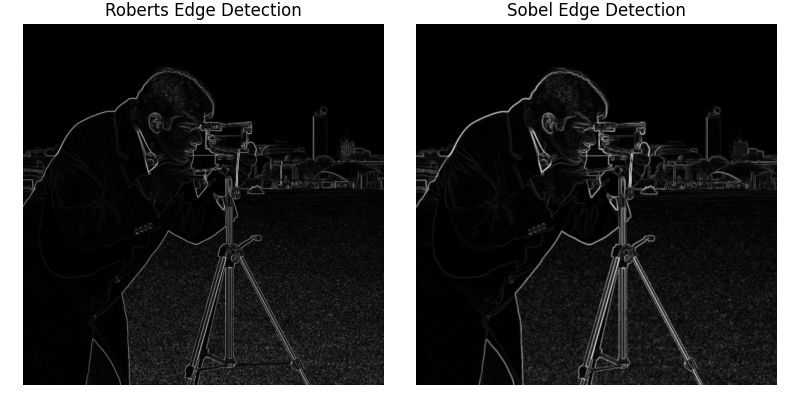
Edge operators are used in image processing within edge detection algorithms. They are discrete differentiation operators, computing an approximation of the gradient of the image intensity function.
import numpy as np
import matplotlib.pyplot as plt

from skimage import filters
from skimage.data import camera
from skimage.util import compare_images


image = camera()
edge_roberts = filters.roberts(image)
edge_sobel = filters.sobel(image)

fig, axes = plt.subplots(ncols=2, sharex=True, sharey=True,
                         figsize=(8, 4))

axes[0].imshow(edge_roberts, cmap=plt.cm.gray)
axes[0].set_title('Roberts Edge Detection')

axes[1].imshow(edge_sobel, cmap=plt.cm.gray)
axes[1].set_title('Sobel Edge Detection')

for ax in axes:
    ax.axis('off')

plt.tight_layout()
plt.show()

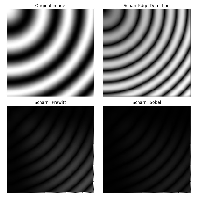
Different operators compute different finite-difference approximations of the gradient. For example, the Scharr filter results in a less rotational variance than the Sobel filter that is in turn better than the Prewitt filter [1] [2] [3]. The difference between the Prewitt and Sobel filters and the Scharr filter is illustrated below with an image that is the discretization of a rotation- invariant continuous function. The discrepancy between the Prewitt and Sobel filters, and the Scharr filter is stronger for regions of the image where the direction of the gradient is close to diagonal, and for regions with high spatial frequencies. For the example image the differences between the filter results are very small and the filter results are visually almost indistinguishable.
x, y = np.ogrid[:100, :100]

# Creating a rotation-invariant image with different spatial frequencies.
image_rot = np.exp(1j * np.hypot(x, y) ** 1.3 / 20.).real

edge_sobel = filters.sobel(image_rot)
edge_scharr = filters.scharr(image_rot)
edge_prewitt = filters.prewitt(image_rot)

diff_scharr_prewitt = compare_images(edge_scharr, edge_prewitt)
diff_scharr_sobel = compare_images(edge_scharr, edge_sobel)
max_diff = np.max(np.maximum(diff_scharr_prewitt, diff_scharr_sobel))

fig, axes = plt.subplots(nrows=2, ncols=2, sharex=True, sharey=True,
                         figsize=(8, 8))
axes = axes.ravel()

axes[0].imshow(image_rot, cmap=plt.cm.gray)
axes[0].set_title('Original image')

axes[1].imshow(edge_scharr, cmap=plt.cm.gray)
axes[1].set_title('Scharr Edge Detection')

axes[2].imshow(diff_scharr_prewitt, cmap=plt.cm.gray, vmax=max_diff)
axes[2].set_title('Scharr - Prewitt')

axes[3].imshow(diff_scharr_sobel, cmap=plt.cm.gray, vmax=max_diff)
axes[3].set_title('Scharr - Sobel')

for ax in axes:
    ax.axis('off')

plt.tight_layout()
plt.show()

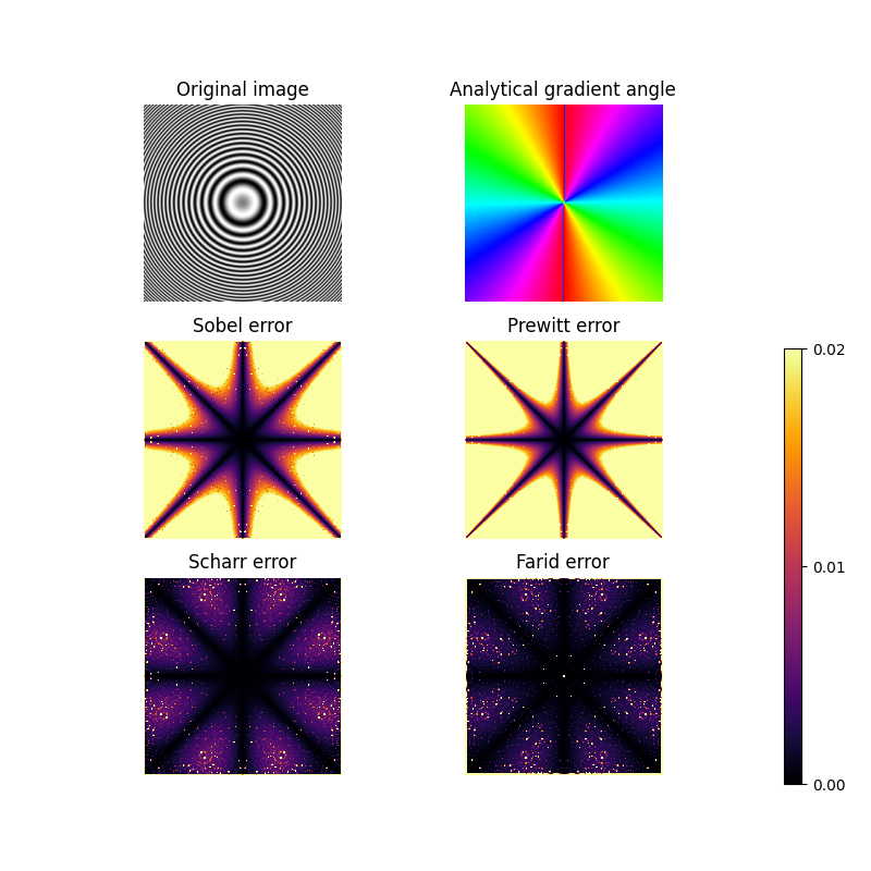
As in the previous example, here we illustrate the rotational invariance of the filters. The top row shows a rotationally invariant image along with the angle of its analytical gradient. The other two rows contain the difference between the different gradient approximations (Sobel, Prewitt, Scharr & Farid) and analytical gradient.
The Farid & Simoncelli derivative filters [4], [5] are the most rotationally invariant, but require a 5x5 kernel, which is computationally more intensive than a 3x3 kernel.
Farid, H. and Simoncelli, E. P., “Differentiation of discrete multidimensional signals”, IEEE Transactions on Image Processing 13(4): 496-508, 2004. DOI:10.1109/TIP.2004.823819
Wikipedia, “Farid and Simoncelli Derivatives.” Available at: <https://en.wikipedia.org/wiki/Image_derivatives#Farid_and_Simoncelli_Derivatives>
x, y = np.mgrid[-10:10:255j, -10:10:255j]
image_rotinv = np.sin(x ** 2 + y ** 2)

image_x = 2 * x * np.cos(x ** 2 + y ** 2)
image_y = 2 * y * np.cos(x ** 2 + y ** 2)

def angle(dx, dy):
    """Calculate the angles between horizontal and vertical operators."""
    return np.mod(np.arctan2(dy, dx), np.pi)


true_angle = angle(image_x, image_y)

angle_farid = angle(filters.farid_h(image_rotinv),
                    filters.farid_v(image_rotinv))
angle_sobel = angle(filters.sobel_h(image_rotinv),
                    filters.sobel_v(image_rotinv))
angle_scharr = angle(filters.scharr_h(image_rotinv),
                     filters.scharr_v(image_rotinv))
angle_prewitt = angle(filters.prewitt_h(image_rotinv),
                      filters.prewitt_v(image_rotinv))

def diff_angle(angle_1, angle_2):
    """Calculate the differences between two angles."""
    return np.minimum(np.pi - np.abs(angle_1 - angle_2),
                      np.abs(angle_1 - angle_2))


diff_farid = diff_angle(true_angle, angle_farid)
diff_sobel = diff_angle(true_angle, angle_sobel)
diff_scharr = diff_angle(true_angle, angle_scharr)
diff_prewitt = diff_angle(true_angle, angle_prewitt)

fig, axes = plt.subplots(nrows=3, ncols=2, sharex=True, sharey=True,
                         figsize=(8, 8))
axes = axes.ravel()

axes[0].imshow(image_rotinv, cmap=plt.cm.gray)
axes[0].set_title('Original image')

axes[1].imshow(true_angle, cmap=plt.cm.hsv)
axes[1].set_title('Analytical gradient angle')

axes[2].imshow(diff_sobel, cmap=plt.cm.inferno, vmin=0, vmax=0.02)
axes[2].set_title('Sobel error')

axes[3].imshow(diff_prewitt, cmap=plt.cm.inferno, vmin=0, vmax=0.02)
axes[3].set_title('Prewitt error')

axes[4].imshow(diff_scharr, cmap=plt.cm.inferno, vmin=0, vmax=0.02)
axes[4].set_title('Scharr error')

color_ax = axes[5].imshow(diff_farid, cmap=plt.cm.inferno, vmin=0, vmax=0.02)
axes[5].set_title('Farid error')

fig.subplots_adjust(right=0.8)
colorbar_ax = fig.add_axes([0.90, 0.10, 0.02, 0.50])
fig.colorbar(color_ax, cax=colorbar_ax, ticks=[0, 0.01, 0.02])

for ax in axes:
    ax.axis('off')

plt.show()

Total running time of the script: (0 minutes 2.270 seconds)