Butterworth Filters

The Butterworth filter is implemented in the frequency domain and is designed to have no passband or stopband ripple. It can be used in either a lowpass or highpass variant. The cutoff_frequency_ratio parameter is used to set the cutoff frequency as a fraction of the sampling frequency. Given that the Nyquist frequency is half the sampling frequency, this means that this parameter should be a positive floating point value < 0.5. The order of the filter can be adjusted to control the transition width, with higher values leading to a sharper transition between the passband and stopband.

Butterworth filtering example

Here we define a get_filtered helper function to repeat lowpass and highpass filtering at a specified series of cutoff frequencies.

import matplotlib.pyplot as plt

from skimage import data, filters

image = data.camera()

# cutoff frequencies as a fraction of the maximum frequency
cutoffs = [0.02, 0.08, 0.16]


def get_filtered(image, cutoffs, squared_butterworth=True, order=3.0, npad=0):
    """Lowpass and highpass butterworth filtering at all specified cutoffs.

    Parameters
    ----------
    image : ndarray
        The image to be filtered.
    cutoffs : sequence of int
        Both lowpass and highpass filtering will be performed for each cutoff
        frequency in `cutoffs`.
    squared_butterworth : bool, optional
        Whether the traditional Butterworth filter or its square is used.
    order : float, optional
        The order of the Butterworth filter

    Returns
    -------
    lowpass_filtered : list of ndarray
        List of images lowpass filtered at the frequencies in `cutoffs`.
    highpass_filtered : list of ndarray
        List of images highpass filtered at the frequencies in `cutoffs`.
    """

    lowpass_filtered = []
    highpass_filtered = []
    for cutoff in cutoffs:
        lowpass_filtered.append(
            filters.butterworth(
                image,
                cutoff_frequency_ratio=cutoff,
                order=order,
                high_pass=False,
                squared_butterworth=squared_butterworth,
                npad=npad,
            )
        )
        highpass_filtered.append(
            filters.butterworth(
                image,
                cutoff_frequency_ratio=cutoff,
                order=order,
                high_pass=True,
                squared_butterworth=squared_butterworth,
                npad=npad,
            )
        )
    return lowpass_filtered, highpass_filtered


def plot_filtered(lowpass_filtered, highpass_filtered, cutoffs):
    """Generate plots for paired lists of lowpass and highpass images."""
    fig, axes = plt.subplots(2, 1 + len(cutoffs), figsize=(12, 8))
    fontdict = dict(fontsize=14, fontweight='bold')

    axes[0, 0].imshow(image, cmap='gray')
    axes[0, 0].set_title('original', fontdict=fontdict)
    axes[1, 0].set_axis_off()

    for i, c in enumerate(cutoffs):
        axes[0, i + 1].imshow(lowpass_filtered[i], cmap='gray')
        axes[0, i + 1].set_title(f'lowpass, c={c}', fontdict=fontdict)
        axes[1, i + 1].imshow(highpass_filtered[i], cmap='gray')
        axes[1, i + 1].set_title(f'highpass, c={c}', fontdict=fontdict)

    for ax in axes.ravel():
        ax.set_xticks([])
        ax.set_yticks([])
    plt.tight_layout()
    return fig, axes


# Perform filtering with the (squared) Butterworth filter at a range of
# cutoffs.
lowpasses, highpasses = get_filtered(image, cutoffs, squared_butterworth=True)

fig, axes = plot_filtered(lowpasses, highpasses, cutoffs)
titledict = dict(fontsize=18, fontweight='bold')
fig.text(
    0.5,
    0.95,
    '(squared) Butterworth filtering (order=3.0, npad=0)',
    fontdict=titledict,
    horizontalalignment='center',
)

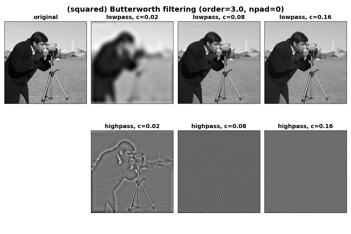
Text(0.5, 0.95, '(squared) Butterworth filtering (order=3.0, npad=0)')

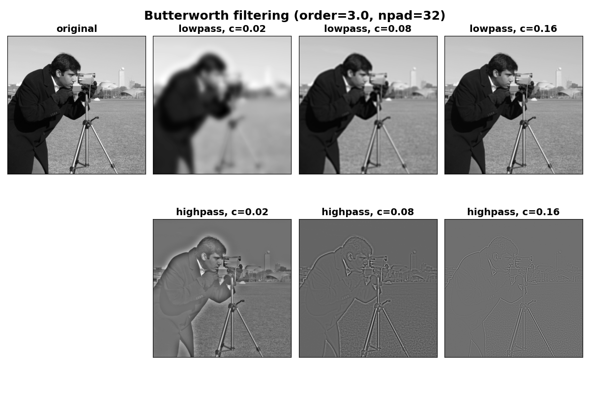
Avoiding boundary artifacts

It can be seen in the images above that there are artifacts near the edge of the images (particularly for the smaller cutoff values). This is due to the periodic nature of the DFT and can be reduced by applying some amount of padding to the edges prior to filtering so that there are not sharp eges in the periodic extension of the image. This can be done via the npad argument to butterworth.

Note that with padding, the undesired shading at the image edges is substantially reduced.

lowpasses, highpasses = get_filtered(image, cutoffs, squared_butterworth=True, npad=32)

fig, axes = plot_filtered(lowpasses, highpasses, cutoffs)
fig.text(
    0.5,
    0.95,
    '(squared) Butterworth filtering (order=3.0, npad=32)',
    fontdict=titledict,
    horizontalalignment='center',
)

Text(0.5, 0.95, '(squared) Butterworth filtering (order=3.0, npad=32)')

True Butterworth filter

To use the traditional signal processing definition of the Butterworth filter, set squared_butterworth=False. This variant has an amplitude profile in the frequency domain that is the square root of the default case. This causes the transition from the passband to the stopband to be more gradual at any given order. This can be seen in the following images which appear a bit sharper in the lowpass case than their squared Butterworth counterparts above.

lowpasses, highpasses = get_filtered(image, cutoffs, squared_butterworth=False, npad=32)

fig, axes = plot_filtered(lowpasses, highpasses, cutoffs)
fig.text(
    0.5,
    0.95,
    'Butterworth filtering (order=3.0, npad=32)',
    fontdict=titledict,
    horizontalalignment='center',
)

plt.show()