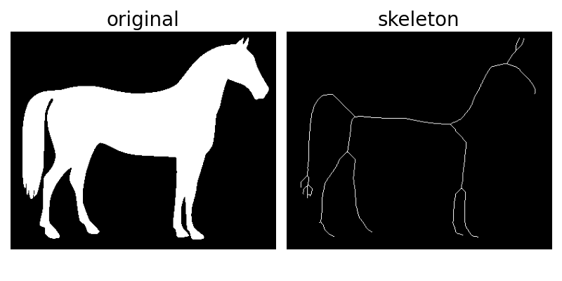
Skeletonize

Skeletonization reduces binary objects to 1 pixel wide representations. This can be useful for feature extraction, and/or representing an object’s topology.

skeletonize works by making successive passes of the image. On each pass, border pixels are identified and removed on the condition that they do not break the connectivity of the corresponding object.

from skimage.morphology import skeletonize
from skimage import data
import matplotlib.pyplot as plt
from skimage.util import invert

# Invert the horse image
image = invert(data.horse())

# perform skeletonization
skeleton = skeletonize(image)

# display results
fig, axes = plt.subplots(nrows=1, ncols=2, figsize=(8, 4), sharex=True, sharey=True)

ax = axes.ravel()

ax[0].imshow(image, cmap=plt.cm.gray)
ax[0].axis('off')
ax[0].set_title('original', fontsize=20)

ax[1].imshow(skeleton, cmap=plt.cm.gray)
ax[1].axis('off')
ax[1].set_title('skeleton', fontsize=20)

fig.tight_layout()
plt.show()

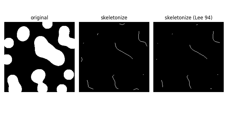
Zhang’s method vs Lee’s method

skeletonize [Zha84] works by making successive passes of the image, removing pixels on object borders. This continues until no more pixels can be removed. The image is correlated with a mask that assigns each pixel a number in the range [0…255] corresponding to each possible pattern of its 8 neighboring pixels. A look up table is then used to assign the pixels a value of 0, 1, 2 or 3, which are selectively removed during the iterations.

skeletonize(..., method='lee') [Lee94] uses an octree data structure to examine a 3x3x3 neighborhood of a pixel. The algorithm proceeds by iteratively sweeping over the image, and removing pixels at each iteration until the image stops changing. Each iteration consists of two steps: first, a list of candidates for removal is assembled; then pixels from this list are rechecked sequentially, to better preserve connectivity of the image.

Note that Lee’s method [Lee94] is designed to be used on 3-D images, and is selected automatically for those. For illustrative purposes, we apply this algorithm to a 2-D image.

[Zha84]

A fast parallel algorithm for thinning digital patterns, T. Y. Zhang and C. Y. Suen, Communications of the ACM, March 1984, Volume 27, Number 3.

[Lee94] (1,2)

T.-C. Lee, R.L. Kashyap and C.-N. Chu, Building skeleton models via 3-D medial surface/axis thinning algorithms. Computer Vision, Graphics, and Image Processing, 56(6):462-478, 1994.

import matplotlib.pyplot as plt
from skimage.morphology import skeletonize

blobs = data.binary_blobs(200, blob_size_fraction=0.2, volume_fraction=0.35, rng=1)

skeleton = skeletonize(blobs)
skeleton_lee = skeletonize(blobs, method='lee')

fig, axes = plt.subplots(1, 3, figsize=(8, 4), sharex=True, sharey=True)
ax = axes.ravel()

ax[0].imshow(blobs, cmap=plt.cm.gray)
ax[0].set_title('original')
ax[0].axis('off')

ax[1].imshow(skeleton, cmap=plt.cm.gray)
ax[1].set_title('skeletonize')
ax[1].axis('off')

ax[2].imshow(skeleton_lee, cmap=plt.cm.gray)
ax[2].set_title('skeletonize (Lee 94)')
ax[2].axis('off')

fig.tight_layout()
plt.show()

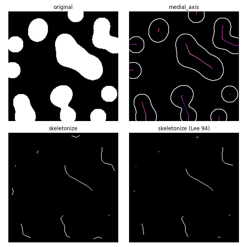
Medial axis skeletonization

The medial axis of an object is the set of all points having more than one closest point on the object’s boundary. It is often called the topological skeleton, because it is a 1-pixel wide skeleton of the object, with the same connectivity as the original object.

Here, we use the medial axis transform to compute the width of the foreground objects. As the function medial_axis returns the distance transform in addition to the medial axis (with the keyword argument return_distance=True), it is possible to compute the distance to the background for all points of the medial axis with this function. This gives an estimate of the local width of the objects.

For a skeleton with fewer branches, skeletonize should be preferred.

from skimage.morphology import medial_axis, skeletonize

# Generate the data
blobs = data.binary_blobs(200, blob_size_fraction=0.2, volume_fraction=0.35, rng=1)

# Compute the medial axis (skeleton) and the distance transform
skel, distance = medial_axis(blobs, return_distance=True)

# Compare with other skeletonization algorithms
skeleton = skeletonize(blobs)
skeleton_lee = skeletonize(blobs, method='lee')

# Distance to the background for pixels of the skeleton
dist_on_skel = distance * skel

fig, axes = plt.subplots(2, 2, figsize=(8, 8), sharex=True, sharey=True)
ax = axes.ravel()

ax[0].imshow(blobs, cmap=plt.cm.gray)
ax[0].set_title('original')
ax[0].axis('off')

ax[1].imshow(dist_on_skel, cmap='magma')
ax[1].contour(blobs, [0.5], colors='w')
ax[1].set_title('medial_axis')
ax[1].axis('off')

ax[2].imshow(skeleton, cmap=plt.cm.gray)
ax[2].set_title('skeletonize')
ax[2].axis('off')

ax[3].imshow(skeleton_lee, cmap=plt.cm.gray)
ax[3].set_title("skeletonize (Lee 94)")
ax[3].axis('off')

fig.tight_layout()
plt.show()

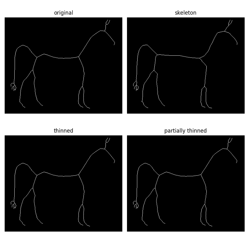
Morphological thinning

Morphological thinning, implemented in the thin function, works on the same principle as skeletonize: remove pixels from the borders at each iteration until none can be removed without altering the connectivity. The different rules of removal can speed up skeletonization and result in different final skeletons.

The thin function also takes an optional max_num_iter keyword argument to limit the number of thinning iterations, and thus produce a relatively thicker skeleton.

from skimage.morphology import skeletonize, thin

skeleton = skeletonize(image)
thinned = thin(image)
thinned_partial = thin(image, max_num_iter=25)

fig, axes = plt.subplots(2, 2, figsize=(8, 8), sharex=True, sharey=True)
ax = axes.ravel()

ax[0].imshow(image, cmap=plt.cm.gray)
ax[0].set_title('original')
ax[0].axis('off')

ax[1].imshow(skeleton, cmap=plt.cm.gray)
ax[1].set_title('skeleton')
ax[1].axis('off')

ax[2].imshow(thinned, cmap=plt.cm.gray)
ax[2].set_title('thinned')
ax[2].axis('off')

ax[3].imshow(thinned_partial, cmap=plt.cm.gray)
ax[3].set_title('partially thinned')
ax[3].axis('off')

fig.tight_layout()
plt.show()