10. Geometrical transformations of images#
10.1. Cropping, resizing and rescaling images#
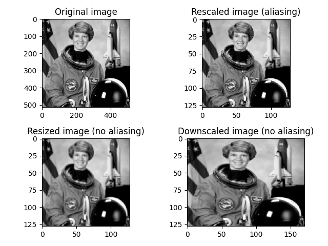
Images being NumPy arrays (as described in the A crash course on NumPy for images section), cropping an image can be done with simple slicing operations. Below we crop a 100x100 square corresponding to the top-left corner of the astronaut image. Note that this operation is done for all color channels (the color dimension is the last, third dimension):
>>> import skimage as ski
>>> img = ski.data.astronaut()
>>> top_left = img[:100, :100]
In order to change the shape of the image, skimage.color provides several
functions described in Rescale, resize, and downscale
.
from skimage import data, color
from skimage.transform import rescale, resize, downscale_local_mean

image = color.rgb2gray(data.astronaut())

image_rescaled = rescale(image, 0.25, anti_aliasing=False)
image_resized = resize(
    image, (image.shape[0] // 4, image.shape[1] // 4), anti_aliasing=True
)
image_downscaled = downscale_local_mean(image, (4, 3))
10.2. Projective transforms (homographies)#
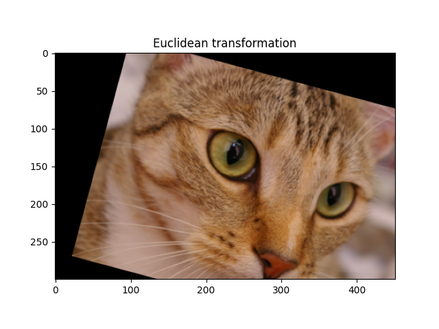
Homographies are transformations of a Euclidean space that preserve the alignment of points. Specific cases of homographies correspond to the conservation of more properties, such as parallelism (affine transformation), shape (similar transformation) or distances (Euclidean transformation). The different types of homographies available in scikit-image are presented in Types of homographies.
Projective transformations can either be created using the explicit parameters (e.g. scale, shear, rotation and translation):
import numpy as np
import skimage as ski

tform = ski.transform.EuclideanTransform(
   rotation=np.pi / 12.,
   translation = (100, -20)
   )
or the full transformation matrix:
matrix = np.array([[np.cos(np.pi/12), -np.sin(np.pi/12), 100],
                   [np.sin(np.pi/12), np.cos(np.pi/12), -20],
                   [0, 0, 1]])
tform = ski.transform.EuclideanTransform(matrix)
The transformation matrix of a transform is available as its tform.params
attribute. Transformations can be composed by multiplying matrices with the
@ matrix multiplication operator.
Transformation matrices use Homogeneous coordinates, which are the extension of Cartesian coordinates used in Euclidean geometry to the more general projective geometry. In particular, points at infinity can be represented with finite coordinates.
Transformations can be applied to images using skimage.transform.warp():
img = ski.util.img_as_float(ski.data.chelsea())
tf_img = ski.transform.warp(img, tform.inverse)
The different transformations in skimage.transform have a
from_estimate class method in order to generate a matching tranform by
estimating the transform parameters from two sets of points (the source and
the destination), as explained in the
Using geometric transformations tutorial:
text = ski.data.text()

src = np.array([[0, 0], [0, 50], [300, 50], [300, 0]])
dst = np.array([[155, 15], [65, 40], [260, 130], [360, 95]])

tform3 = ski.transform.ProjectiveTransform.from_estimate(src, dst)
warped = ski.transform.warp(text, tform3, output_shape=(50, 300))
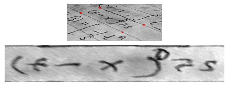
The from_estimate class method uses least squares optimization to minimize
the distance between source and optimization. Source and destination points
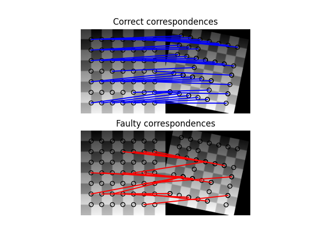
can be determined manually, or using the different methods for feature
detection available in skimage.feature, such as
and matching points using skimage.feature.match_descriptors() before
estimating transformation parameters. However, spurious matches are often made,
and it is advisable to use the RANSAC algorithm (instead of simple
least-squares optimization) to improve the robustness to outliers, as explained
in Robust matching using RANSAC.
Examples showing applications of transformation estimation are
stereo matching Fundamental matrix estimation and
image rectification Using geometric transformations
The from_estimate class method is point-based, that is, it uses only a set
of points from the source and destination images. For estimating translations
(shifts), it is also possible to use a full-field method using all pixels,
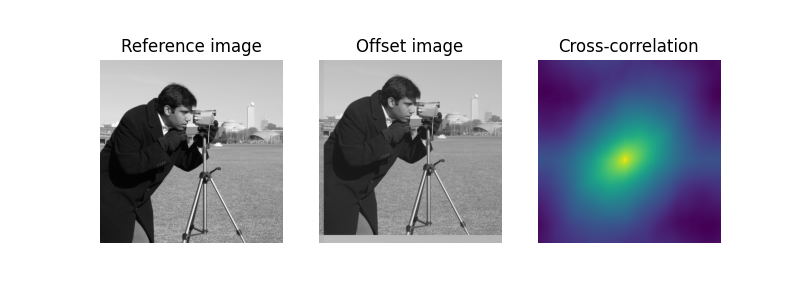
based on Fourier-space cross-correlation. This method is implemented by
skimage.registration.phase_cross_correlation() and explained in the
Image Registration
tutorial.
Bear in mind that the estimation can fail, in which case from_estimate
returns a special FailedEstimation object instead of a valid transform.
See the Using geometric transformations tutorial for
more detail on testing for such estimation failures.
The Using Polar and Log-Polar Transformations for Registration tutorial explains a variant of this full-field method for estimating a rotation, by using first a log-polar transformation.