Module: color <a class="headerlink" href="#module-skimage.color" title="Permalink to this heading">¶

[2]

A. R. Robertson, “The CIE 1976 color-difference formulae,” Color Res. Appl. 2, 7-11 (1977).

deltaE_ciede2000¶

skimage.color.deltaE_ciede2000(lab1, lab2, kL=1, kC=1, kH=1, *, channel_axis=-1)[source]¶

Color difference as given by the CIEDE 2000 standard.

CIEDE 2000 is a major revision of CIDE94. The perceptual calibration is largely based on experience with automotive paint on smooth surfaces.

Parameters:

lab1array_like: reference color (Lab colorspace)
lab2array_like: comparison color (Lab colorspace)
kLfloat (range), optional: lightness scale factor, 1 for “acceptably close”; 2 for “imperceptible” see deltaE_cmc
kCfloat (range), optional: chroma scale factor, usually 1
kHfloat (range), optional: hue scale factor, usually 1
channel_axisint, optional: This parameter indicates which axis of the arrays corresponds to channels.

New in version 0.19: channel_axis was added in 0.19.

Returns:

deltaEarray_like: The distance between lab1 and lab2

Notes

CIEDE 2000 assumes parametric weighting factors for the lightness, chroma, and hue (kL, kC, kH respectively). These default to 1.

References

[1]

http://www.ece.rochester.edu/~gsharma/ciede2000/ciede2000noteCRNA.pdf DOI:10.1364/AO.33.008069

[2]

[3]

M. Melgosa, J. Quesada, and E. Hita, “Uniformity of some recent color metrics tested with an accurate color-difference tolerance dataset,” Appl. Opt. 33, 8069-8077 (1994).

deltaE_ciede94¶

skimage.color.deltaE_ciede94(lab1, lab2, kH=1, kC=1, kL=1, k1=0.045, k2=0.015, *, channel_axis=-1)[source]¶

Color difference according to CIEDE 94 standard

Accommodates perceptual non-uniformities through the use of application specific scale factors (kH, kC, kL, k1, and k2).

Parameters:

lab1array_like: reference color (Lab colorspace)
lab2array_like: comparison color (Lab colorspace)
kHfloat, optional: Hue scale
kCfloat, optional: Chroma scale
kLfloat, optional: Lightness scale
k1float, optional: first scale parameter
k2float, optional: second scale parameter
channel_axisint, optional: This parameter indicates which axis of the arrays corresponds to channels.

New in version 0.19: channel_axis was added in 0.19.

Returns:

dEarray_like: color difference between lab1 and lab2

Notes

deltaE_ciede94 is not symmetric with respect to lab1 and lab2. CIEDE94 defines the scales for the lightness, hue, and chroma in terms of the first color. Consequently, the first color should be regarded as the “reference” color.

kL, k1, k2 depend on the application and default to the values suggested for graphic arts

Parameter	Graphic Arts	Textiles
kL	1.000	2.000
k1	0.045	0.048
k2	0.015	0.014

References

[1]

http://www.brucelindbloom.com/index.html?Eqn_DeltaE_CIE94.html

[2]

deltaE_cmc¶

skimage.color.deltaE_cmc(lab1, lab2, kL=1, kC=1, *, channel_axis=-1)[source]¶

Color difference from the CMC l:c standard.

This color difference was developed by the Colour Measurement Committee (CMC) of the Society of Dyers and Colourists (United Kingdom). It is intended for use in the textile industry.

The scale factors kL, kC set the weight given to differences in lightness and chroma relative to differences in hue. The usual values are kL=2, kC=1 for “acceptability” and kL=1, kC=1 for “imperceptibility”. Colors with dE > 1 are “different” for the given scale factors.

Parameters:

lab1array_like: reference color (Lab colorspace)
lab2array_like: comparison color (Lab colorspace)
channel_axisint, optional: This parameter indicates which axis of the arrays corresponds to channels.

New in version 0.19: channel_axis was added in 0.19.

Returns:

dEarray_like: distance between colors lab1 and lab2

Notes

deltaE_cmc the defines the scales for the lightness, hue, and chroma in terms of the first color. Consequently deltaE_cmc(lab1, lab2) != deltaE_cmc(lab2, lab1)

References

[1]

http://www.brucelindbloom.com/index.html?Eqn_DeltaE_CIE94.html

[2]

[3]

F. J. J. Clarke, R. McDonald, and B. Rigg, “Modification to the JPC79 colour-difference formula,” J. Soc. Dyers Colour. 100, 128-132 (1984).

gray2rgb¶

skimage.color.gray2rgb(image, *, channel_axis=-1)[source]¶

Create an RGB representation of a gray-level image.

Parameters:

imagearray_like: Input image.
channel_axisint, optional: This parameter indicates which axis of the output array will correspond to channels.

Returns:

rgb(…, 3, …) ndarray: RGB image. A new dimension of length 3 is added to input image.

Notes

If the input is a 1-dimensional image of shape (M, ), the output will be shape (M, 3).

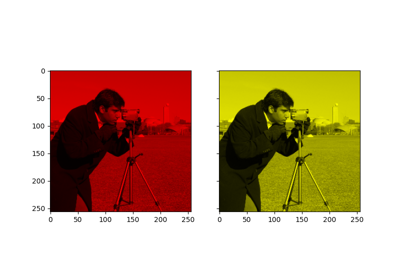
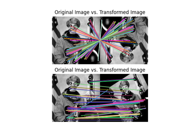
Examples using `skimage.color.gray2rgb`¶

Tinting gray-scale images

Circular and Elliptical Hough Transforms

Region Boundary based RAGs

gray2rgba¶

skimage.color.gray2rgba(image, alpha=None, *, channel_axis=-1)[source]¶

Create a RGBA representation of a gray-level image.

Parameters:

imagearray_like: Input image.
alphaarray_like, optional: Alpha channel of the output image. It may be a scalar or an array that can be broadcast to image. If not specified it is set to the maximum limit corresponding to the image dtype.
channel_axisint, optional: This parameter indicates which axis of the output array will correspond to channels.

New in version 0.19: channel_axis was added in 0.19.

Returns:

rgbandarray: RGBA image. A new dimension of length 4 is added to input image shape.

hed2rgb¶

skimage.color.hed2rgb(hed, *, channel_axis=-1)[source]¶

Haematoxylin-Eosin-DAB (HED) to RGB color space conversion.

Parameters:

hed(…, 3, …) array_like: The image in the HED color space. By default, the final dimension denotes channels.
channel_axisint, optional: This parameter indicates which axis of the array corresponds to channels.

New in version 0.19: channel_axis was added in 0.19.

Returns:

out(…, 3, …) ndarray: The image in RGB. Same dimensions as input.

Raises:

ValueError: If hed is not at least 2-D with shape (…, 3, …).

References

[1]

A. C. Ruifrok and D. A. Johnston, “Quantification of histochemical staining by color deconvolution.,” Analytical and quantitative cytology and histology / the International Academy of Cytology [and] American Society of Cytology, vol. 23, no. 4, pp. 291-9, Aug. 2001.

Examples

>>> from skimage import data
>>> from skimage.color import rgb2hed, hed2rgb
>>> ihc = data.immunohistochemistry()
>>> ihc_hed = rgb2hed(ihc)
>>> ihc_rgb = hed2rgb(ihc_hed)

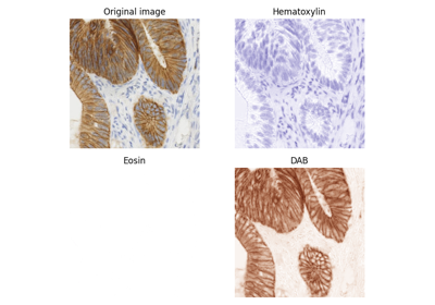
Examples using `skimage.color.hed2rgb`¶

Separate colors in immunohistochemical staining

hsv2rgb¶

skimage.color.hsv2rgb(hsv, *, channel_axis=-1)[source]¶

HSV to RGB color space conversion.

Parameters:

hsv(…, 3, …) array_like: The image in HSV format. By default, the final dimension denotes channels.
channel_axisint, optional: This parameter indicates which axis of the array corresponds to channels.

New in version 0.19: channel_axis was added in 0.19.

Returns:

out(…, 3, …) ndarray: The image in RGB format. Same dimensions as input.

Raises:

ValueError: If hsv is not at least 2-D with shape (…, 3, …).

Notes

Conversion between RGB and HSV color spaces results in some loss of precision, due to integer arithmetic and rounding [1].

References

[1]

https://en.wikipedia.org/wiki/HSL_and_HSV

Examples

>>> from skimage import data
>>> img = data.astronaut()
>>> img_hsv = rgb2hsv(img)
>>> img_rgb = hsv2rgb(img_hsv)

Examples using `skimage.color.hsv2rgb`¶

Tinting gray-scale images

Flood Fill

lab2lch¶

skimage.color.lab2lch(lab, *, channel_axis=-1)[source]¶

Convert image in CIE-LAB to CIE-LCh color space.

CIE-LCh is the cylindrical representation of the CIE-LAB (Cartesian) color space.

Parameters:

lab(…, 3, …) array_like: The input image in CIE-LAB color space. Unless channel_axis is set, the final dimension denotes the CIE-LAB channels. The L* values range from 0 to 100; the a* and b* values range from -128 to 127.
channel_axisint, optional: This parameter indicates which axis of the array corresponds to channels.

New in version 0.19: channel_axis was added in 0.19.

Returns:

out(…, 3, …) ndarray: The image in CIE-LCh color space, of same shape as input.

Raises:

ValueError: If lab does not have at least 3 channels (i.e., L*, a*, and b*).

See also

lch2lab

Notes

The h channel (i.e., hue) is expressed as an angle in range (0, 2*pi).

References

[1]

[2]

https://en.wikipedia.org/wiki/HCL_color_space

[3]

Examples

>>> from skimage import data
>>> from skimage.color import rgb2lab, lab2lch
>>> img = data.astronaut()
>>> img_lab = rgb2lab(img)
>>> img_lch = lab2lch(img_lab)

lab2rgb¶

skimage.color.lab2rgb(lab, illuminant='D65', observer='2', *, channel_axis=-1)[source]¶

Convert image in CIE-LAB to sRGB color space.

Parameters:

lab(…, 3, …) array_like: The input image in CIE-LAB color space. Unless channel_axis is set, the final dimension denotes the CIE-LAB channels. The L* values range from 0 to 100; the a* and b* values range from -128 to 127.
illuminant{“A”, “B”, “C”, “D50”, “D55”, “D65”, “D75”, “E”}, optional: The name of the illuminant (the function is NOT case sensitive).
observer{“2”, “10”, “R”}, optional: The aperture angle of the observer.
channel_axisint, optional: This parameter indicates which axis of the array corresponds to channels.

New in version 0.19: channel_axis was added in 0.19.

Returns:

out(…, 3, …) ndarray: The image in sRGB color space, of same shape as input.

Raises:

ValueError: If lab is not at least 2-D with shape (…, 3, …).

See also

rgb2lab

Notes

This function uses lab2xyz() and xyz2rgb(). The CIE XYZ tristimulus values are x_ref = 95.047, y_ref = 100., and z_ref = 108.883. See function get_xyz_coords() for a list of supported illuminants.

References

[1]

https://en.wikipedia.org/wiki/Standard_illuminant

[2]

lab2xyz¶

skimage.color.lab2xyz(lab, illuminant='D65', observer='2', *, channel_axis=-1)[source]¶

Convert image in CIE-LAB to XYZ color space.

Parameters:

lab(…, 3, …) array_like: The input image in CIE-LAB color space. Unless channel_axis is set, the final dimension denotes the CIE-LAB channels. The L* values range from 0 to 100; the a* and b* values range from -128 to 127.
illuminant{“A”, “B”, “C”, “D50”, “D55”, “D65”, “D75”, “E”}, optional: The name of the illuminant (the function is NOT case sensitive).
observer{“2”, “10”, “R”}, optional: The aperture angle of the observer.
channel_axisint, optional: This parameter indicates which axis of the array corresponds to channels.

New in version 0.19: channel_axis was added in 0.19.

Returns:

out(…, 3, …) ndarray: The image in XYZ color space, of same shape as input.

Raises:

ValueError: If lab is not at least 2-D with shape (…, 3, …).
ValueError: If either the illuminant or the observer angle are not supported or unknown.
UserWarning: If any of the pixels are invalid (Z < 0).

See also

xyz2lab

Notes

The CIE XYZ tristimulus values are x_ref = 95.047, y_ref = 100., and z_ref = 108.883. See function get_xyz_coords() for a list of supported illuminants.

References

[1]

[2]

Local Binary Pattern for texture classification

label2rgb¶

skimage.color.label2rgb(label, image=None, colors=None, alpha=0.3, bg_label=0, bg_color=(0, 0, 0), image_alpha=1, kind='overlay', *, saturation=0, channel_axis=-1)[source]¶

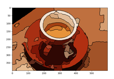
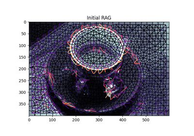
Return an RGB image where color-coded labels are painted over the image.

Parameters:

labelndarray: Integer array of labels with the same shape as image.
imagendarray, optional: Image used as underlay for labels. It should have the same shape as labels, optionally with an additional RGB (channels) axis. If image is an RGB image, it is converted to grayscale before coloring.
colorslist, optional: List of colors. If the number of labels exceeds the number of colors, then the colors are cycled.
alphafloat [0, 1], optional: Opacity of colorized labels. Ignored if image is None.
bg_labelint, optional: Label that’s treated as the background. If bg_label is specified, bg_color is None, and kind is overlay, background is not painted by any colors.
bg_colorstr or array, optional: Background color. Must be a name in color_dict or RGB float values between [0, 1].
image_alphafloat [0, 1], optional: Opacity of the image.
kindstring, one of {‘overlay’, ‘avg’}: The kind of color image desired. ‘overlay’ cycles over defined colors and overlays the colored labels over the original image. ‘avg’ replaces each labeled segment with its average color, for a stained-class or pastel painting appearance.
saturationfloat [0, 1], optional: Parameter to control the saturation applied to the original image between fully saturated (original RGB, saturation=1) and fully unsaturated (grayscale, saturation=0). Only applies when kind=’overlay’.
channel_axisint, optional: This parameter indicates which axis of the output array will correspond to channels. If image is provided, this must also match the axis of image that corresponds to channels.

New in version 0.19: channel_axis was added in 0.19.

Returns:

resultndarray of float, same shape as image: The result of blending a cycling colormap (colors) for each distinct value in label with the image, at a certain alpha value.

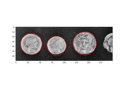
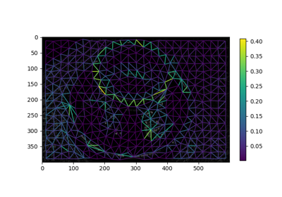
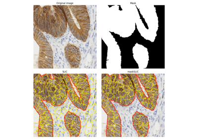
Examples using `skimage.color.label2rgb`¶

RAG Thresholding

Normalized Cut

Find Regular Segments Using Compact Watershed

Expand segmentation labels without overlap

Label image regions

Find the intersection of two segmentations

RAG Merging

Hierarchical Merging of Region Boundary RAGs

Extrema

Use pixel graphs to find an object’s geodesic center

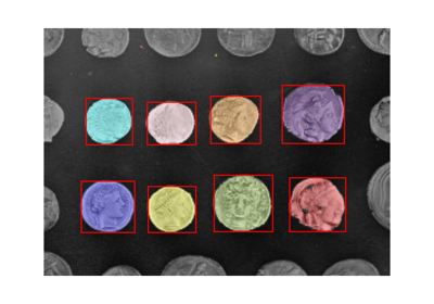
Use pixel graphs to find an object's geodesic center

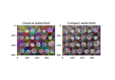
Comparing edge-based and region-based segmentation

Segment human cells (in mitosis)

lch2lab¶

skimage.color.lch2lab(lch, *, channel_axis=-1)[source]¶

Convert image in CIE-LCh to CIE-LAB color space.

CIE-LCh is the cylindrical representation of the CIE-LAB (Cartesian) color space.

Parameters:

lch(…, 3, …) array_like: The input image in CIE-LCh color space. Unless channel_axis is set, the final dimension denotes the CIE-LAB channels. The L* values range from 0 to 100; the C values range from 0 to 100; the h values range from 0 to 2*pi.
channel_axisint, optional: This parameter indicates which axis of the array corresponds to channels.

New in version 0.19: channel_axis was added in 0.19.

Returns:

out(…, 3, …) ndarray: The image in CIE-LAB format, of same shape as input.

Raises:

ValueError: If lch does not have at least 3 channels (i.e., L*, C, and h).

See also

lab2lch

Notes

The h channel (i.e., hue) is expressed as an angle in range (0, 2*pi).

References

[1]

https://en.wikipedia.org/wiki/HCL_color_space

[2]

[3]

http://poynton.ca/PDFs/ColorFAQ.pdf

Examples

>>> from skimage import data
>>> from skimage.color import rgb2lab, lch2lab, lab2lch
>>> img = data.astronaut()
>>> img_lab = rgb2lab(img)
>>> img_lch = lab2lch(img_lab)
>>> img_lab2 = lch2lab(img_lch)

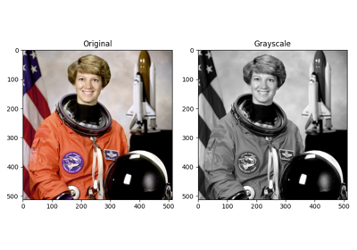
rgb2gray¶

skimage.color.rgb2gray(rgb, *, channel_axis=-1)[source]¶

Compute luminance of an RGB image.

Parameters:

rgb(…, 3, …) array_like: The image in RGB format. By default, the final dimension denotes channels.

Returns:

outndarray: The luminance image - an array which is the same size as the input array, but with the channel dimension removed.

Raises:

ValueError: If rgb is not at least 2-D with shape (…, 3, …).

Notes

The weights used in this conversion are calibrated for contemporary CRT phosphors:

Y = 0.2125 R + 0.7154 G + 0.0721 B

If there is an alpha channel present, it is ignored.

References

[1]

Examples

>>> from skimage.color import rgb2gray
>>> from skimage import data
>>> img = data.astronaut()
>>> img_gray = rgb2gray(img)

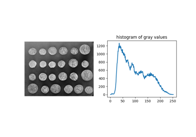
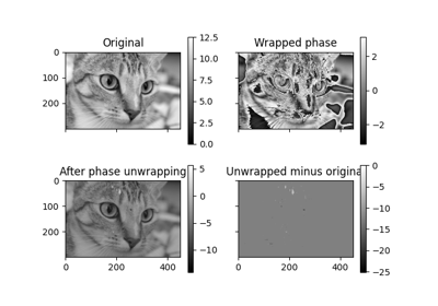
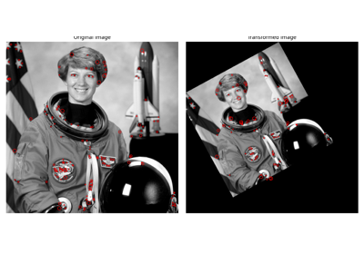
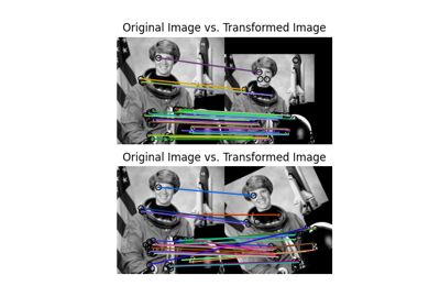
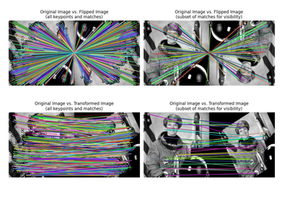
Examples using `skimage.color.rgb2gray`¶

Block views on images/arrays

RGB to grayscale

Adapting gray-scale filters to RGB images

Ridge operators

Active Contour Model

Circular and Elliptical Hough Transforms

Rescale, resize, and downscale

Fundamental matrix estimation

Robust matching using RANSAC

Registration using optical flow

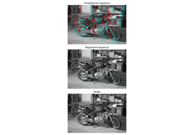
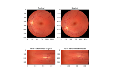
Using Polar and Log-Polar Transformations for Registration

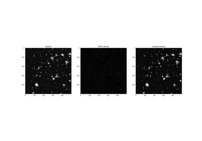
Removing small objects in grayscale images with a top hat filter

Image Deconvolution

Using window functions with images

Image Deconvolution

Estimate strength of blur

Phase Unwrapping

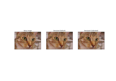
Full tutorial on calibrating Denoisers Using J-Invariance

CENSURE feature detector

Blob Detection

ORB feature detector and binary descriptor

Gabors / Primary Visual Cortex “Simple Cells” from an Image

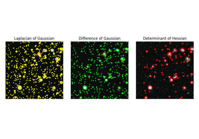
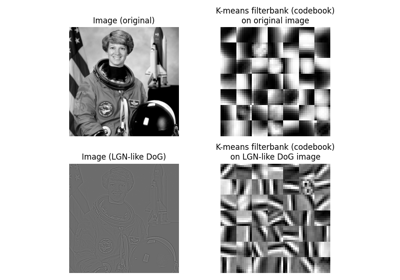
Gabors / Primary Visual Cortex "Simple Cells" from an Image

BRIEF binary descriptor

SIFT feature detector and descriptor extractor

Region Boundary based RAGs

Apply maskSLIC vs SLIC

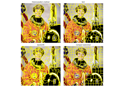
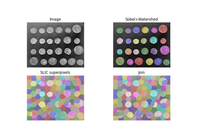
Comparison of segmentation and superpixel algorithms

Hierarchical Merging of Region Boundary RAGs

Extrema

Use pixel graphs to find an object’s geodesic center

Use pixel graphs to find an object's geodesic center

rgb2hed¶

skimage.color.rgb2hed(rgb, *, channel_axis=-1)[source]¶

RGB to Haematoxylin-Eosin-DAB (HED) color space conversion.

Parameters:

rgb(…, 3, …) array_like: The image in RGB format. By default, the final dimension denotes channels.
channel_axisint, optional: This parameter indicates which axis of the array corresponds to channels.

New in version 0.19: channel_axis was added in 0.19.

Returns:

out(…, 3, …) ndarray: The image in HED format. Same dimensions as input.

Raises:

ValueError: If rgb is not at least 2-D with shape (…, 3, …).

References

[1]

Examples

>>> from skimage import data
>>> from skimage.color import rgb2hed
>>> ihc = data.immunohistochemistry()
>>> ihc_hed = rgb2hed(ihc)

Examples using `skimage.color.rgb2hed`¶

Separate colors in immunohistochemical staining

rgb2hsv¶

skimage.color.rgb2hsv(rgb, *, channel_axis=-1)[source]¶

RGB to HSV color space conversion.

Parameters:

rgb(…, 3, …) array_like: The image in RGB format. By default, the final dimension denotes channels.
channel_axisint, optional: This parameter indicates which axis of the array corresponds to channels.

New in version 0.19: channel_axis was added in 0.19.

Returns:

out(…, 3, …) ndarray: The image in HSV format. Same dimensions as input.

Raises:

ValueError: If rgb is not at least 2-D with shape (…, 3, …).

Notes

Conversion between RGB and HSV color spaces results in some loss of precision, due to integer arithmetic and rounding [1].

References

[1]

https://en.wikipedia.org/wiki/HSL_and_HSV

Examples

>>> from skimage import color
>>> from skimage import data
>>> img = data.astronaut()
>>> img_hsv = color.rgb2hsv(img)

Examples using `skimage.color.rgb2hsv`¶

RGB to HSV

Tinting gray-scale images

Flood Fill

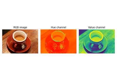
rgb2lab¶

skimage.color.rgb2lab(rgb, illuminant='D65', observer='2', *, channel_axis=-1)[source]¶

Conversion from the sRGB color space (IEC 61966-2-1:1999) to the CIE Lab colorspace under the given illuminant and observer.

Parameters:

rgb(…, 3, …) array_like: The image in RGB format. By default, the final dimension denotes channels.
illuminant{“A”, “B”, “C”, “D50”, “D55”, “D65”, “D75”, “E”}, optional: The name of the illuminant (the function is NOT case sensitive).
observer{“2”, “10”, “R”}, optional: The aperture angle of the observer.
channel_axisint, optional: This parameter indicates which axis of the array corresponds to channels.

New in version 0.19: channel_axis was added in 0.19.

Returns:

out(…, 3, …) ndarray: The image in Lab format. Same dimensions as input.

Raises:

ValueError: If rgb is not at least 2-D with shape (…, 3, …).

Notes

RGB is a device-dependent color space so, if you use this function, be sure that the image you are analyzing has been mapped to the sRGB color space.

This function uses rgb2xyz and xyz2lab. By default Observer=”2”, Illuminant=”D65”. CIE XYZ tristimulus values x_ref=95.047, y_ref=100., z_ref=108.883. See function get_xyz_coords for a list of supported illuminants.

References

[1]

https://en.wikipedia.org/wiki/Standard_illuminant

rgb2rgbcie¶

skimage.color.rgb2rgbcie(rgb, *, channel_axis=-1)[source]¶

RGB to RGB CIE color space conversion.

Parameters:

rgb(…, 3, …) array_like: The image in RGB format. By default, the final dimension denotes channels.
channel_axisint, optional: This parameter indicates which axis of the array corresponds to channels.

New in version 0.19: channel_axis was added in 0.19.

Returns:

out(…, 3, …) ndarray: The image in RGB CIE format. Same dimensions as input.

Raises:

ValueError: If rgb is not at least 2-D with shape (…, 3, …).

References

[1]

Examples

>>> from skimage import data
>>> from skimage.color import rgb2rgbcie
>>> img = data.astronaut()
>>> img_rgbcie = rgb2rgbcie(img)

rgb2xyz¶

skimage.color.rgb2xyz(rgb, *, channel_axis=-1)[source]¶

RGB to XYZ color space conversion.

Parameters:

rgb(…, 3, …) array_like: The image in RGB format. By default, the final dimension denotes channels.
channel_axisint, optional: This parameter indicates which axis of the array corresponds to channels.

New in version 0.19: channel_axis was added in 0.19.

Returns:

out(…, 3, …) ndarray: The image in XYZ format. Same dimensions as input.

Raises:

ValueError: If rgb is not at least 2-D with shape (…, 3, …).

Notes

The CIE XYZ color space is derived from the CIE RGB color space. Note however that this function converts from sRGB.

References

[1]

https://en.wikipedia.org/wiki/YCbCr

Examples

>>> from skimage import data
>>> img = data.astronaut()
>>> img_xyz = rgb2xyz(img)

rgb2ycbcr¶

skimage.color.rgb2ycbcr(rgb, *, channel_axis=-1)[source]¶

RGB to YCbCr color space conversion.

Parameters:

rgb(…, 3, …) array_like: The image in RGB format. By default, the final dimension denotes channels.
channel_axisint, optional: This parameter indicates which axis of the array corresponds to channels.

New in version 0.19: channel_axis was added in 0.19.

Returns:

out(…, 3, …) ndarray: The image in YCbCr format. Same dimensions as input.

Raises:

ValueError: If rgb is not at least 2-D with shape (…, 3, …).

Notes

Y is between 16 and 235. This is the color space commonly used by video codecs; it is sometimes incorrectly called “YUV”.

References

[1]

rgb2ydbdr¶

skimage.color.rgb2ydbdr(rgb, *, channel_axis=-1)[source]¶

RGB to YDbDr color space conversion.

Parameters:

rgb(…, 3, …) array_like: The image in RGB format. By default, the final dimension denotes channels.
channel_axisint, optional: This parameter indicates which axis of the array corresponds to channels.

New in version 0.19: channel_axis was added in 0.19.

Returns:

out(…, 3, …) ndarray: The image in YDbDr format. Same dimensions as input.

Raises:

ValueError: If rgb is not at least 2-D with shape (…, 3, …).

Notes

This is the color space commonly used by video codecs. It is also the reversible color transform in JPEG2000.

References

[1]

https://en.wikipedia.org/wiki/YDbDr

rgb2yiq¶

skimage.color.rgb2yiq(rgb, *, channel_axis=-1)[source]¶

RGB to YIQ color space conversion.

Parameters:

rgb(…, 3, …) array_like: The image in RGB format. By default, the final dimension denotes channels.
channel_axisint, optional: This parameter indicates which axis of the array corresponds to channels.

New in version 0.19: channel_axis was added in 0.19.

Returns:

out(…, 3, …) ndarray: The image in YIQ format. Same dimensions as input.

Raises:

ValueError: If rgb is not at least 2-D with shape (…, 3, …).

rgb2ypbpr¶

skimage.color.rgb2ypbpr(rgb, *, channel_axis=-1)[source]¶

RGB to YPbPr color space conversion.

Parameters:

rgb(…, 3, …) array_like: The image in RGB format. By default, the final dimension denotes channels.
channel_axisint, optional: This parameter indicates which axis of the array corresponds to channels.

New in version 0.19: channel_axis was added in 0.19.

Returns:

out(…, 3, …) ndarray: The image in YPbPr format. Same dimensions as input.

Raises:

ValueError: If rgb is not at least 2-D with shape (…, 3, …).

References

[1]

https://en.wikipedia.org/wiki/YPbPr

rgb2yuv¶

skimage.color.rgb2yuv(rgb, *, channel_axis=-1)[source]¶

RGB to YUV color space conversion.

Parameters:

rgb(…, 3, …) array_like: The image in RGB format. By default, the final dimension denotes channels.
channel_axisint, optional: This parameter indicates which axis of the array corresponds to channels.

New in version 0.19: channel_axis was added in 0.19.

Returns:

out(…, 3, …) ndarray: The image in YUV format. Same dimensions as input.

Raises:

ValueError: If rgb is not at least 2-D with shape (…, 3, …).

Notes

Y is between 0 and 1. Use YCbCr instead of YUV for the color space commonly used by video codecs, where Y ranges from 16 to 235.

References

[1]

https://en.wikipedia.org/wiki/YUV

rgba2rgb¶

skimage.color.rgba2rgb(rgba, background=(1, 1, 1), *, channel_axis=-1)[source]¶

RGBA to RGB conversion using alpha blending [1].

Parameters:

rgba(…, 4, …) array_like: The image in RGBA format. By default, the final dimension denotes channels.
backgroundarray_like: The color of the background to blend the image with (3 floats between 0 to 1 - the RGB value of the background).
channel_axisint, optional: This parameter indicates which axis of the array corresponds to channels.

New in version 0.19: channel_axis was added in 0.19.

Returns:

out(…, 3, …) ndarray: The image in RGB format. Same dimensions as input.

Raises:

ValueError: If rgba is not at least 2D with shape (…, 4, …).

References

[1] (1,2)

https://en.wikipedia.org/wiki/Alpha_compositing#Alpha_blending

Examples

>>> from skimage import color
>>> from skimage import data
>>> img_rgba = data.logo()
>>> img_rgb = color.rgba2rgb(img_rgba)

rgbcie2rgb¶

skimage.color.rgbcie2rgb(rgbcie, *, channel_axis=-1)[source]¶

RGB CIE to RGB color space conversion.

Parameters:

rgbcie(…, 3, …) array_like: The image in RGB CIE format. By default, the final dimension denotes channels.
channel_axisint, optional: This parameter indicates which axis of the array corresponds to channels.

New in version 0.19: channel_axis was added in 0.19.

Returns:

out(…, 3, …) ndarray: The image in RGB format. Same dimensions as input.

Raises:

ValueError: If rgbcie is not at least 2-D with shape (…, 3, …).

References

[1]

https://web.archive.org/web/20160624145052/http://www.mecourse.com/landinig/software/cdeconv/cdeconv.html

Examples

>>> from skimage import data
>>> from skimage.color import rgb2rgbcie, rgbcie2rgb
>>> img = data.astronaut()
>>> img_rgbcie = rgb2rgbcie(img)
>>> img_rgb = rgbcie2rgb(img_rgbcie)

separate_stains¶

skimage.color.separate_stains(rgb, conv_matrix, *, channel_axis=-1)[source]¶

RGB to stain color space conversion.

Parameters:

rgb(…, 3, …) array_like: The image in RGB format. By default, the final dimension denotes channels.
conv_matrix: ndarray: The stain separation matrix as described by G. Landini [1].
channel_axisint, optional: This parameter indicates which axis of the array corresponds to channels.

New in version 0.19: channel_axis was added in 0.19.

Returns:

out(…, 3, …) ndarray: The image in stain color space. Same dimensions as input.

Raises:

ValueError: If rgb is not at least 2-D with shape (…, 3, …).

Notes

Stain separation matrices available in the color module and their respective colorspace:

hed_from_rgb: Hematoxylin + Eosin + DAB
hdx_from_rgb: Hematoxylin + DAB
fgx_from_rgb: Feulgen + Light Green
bex_from_rgb: Giemsa stain : Methyl Blue + Eosin
rbd_from_rgb: FastRed + FastBlue + DAB
gdx_from_rgb: Methyl Green + DAB
hax_from_rgb: Hematoxylin + AEC
bro_from_rgb: Blue matrix Anilline Blue + Red matrix Azocarmine + Orange matrix Orange-G
bpx_from_rgb: Methyl Blue + Ponceau Fuchsin
ahx_from_rgb: Alcian Blue + Hematoxylin
hpx_from_rgb: Hematoxylin + PAS

This implementation borrows some ideas from DIPlib [2], e.g. the compensation using a small value to avoid log artifacts when calculating the Beer-Lambert law.

References

[1]

[2]

https://github.com/DIPlib/diplib/

[3]

A. C. Ruifrok and D. A. Johnston, “Quantification of histochemical staining by color deconvolution,” Anal. Quant. Cytol. Histol., vol. 23, no. 4, pp. 291–299, Aug. 2001.

Examples

>>> from skimage import data
>>> from skimage.color import separate_stains, hdx_from_rgb
>>> ihc = data.immunohistochemistry()
>>> ihc_hdx = separate_stains(ihc, hdx_from_rgb)

xyz2lab¶

skimage.color.xyz2lab(xyz, illuminant='D65', observer='2', *, channel_axis=-1)[source]¶

XYZ to CIE-LAB color space conversion.

Parameters:

xyz(…, 3, …) array_like: The image in XYZ format. By default, the final dimension denotes channels.
illuminant{“A”, “B”, “C”, “D50”, “D55”, “D65”, “D75”, “E”}, optional: The name of the illuminant (the function is NOT case sensitive).
observer{“2”, “10”, “R”}, optional: One of: 2-degree observer, 10-degree observer, or ‘R’ observer as in R function grDevices::convertColor.
channel_axisint, optional: This parameter indicates which axis of the array corresponds to channels.

New in version 0.19: channel_axis was added in 0.19.

Returns:

out(…, 3, …) ndarray: The image in CIE-LAB format. Same dimensions as input.

Raises:

ValueError: If xyz is not at least 2-D with shape (…, 3, …).
ValueError: If either the illuminant or the observer angle is unsupported or unknown.

Notes

By default Observer=”2”, Illuminant=”D65”. CIE XYZ tristimulus values x_ref=95.047, y_ref=100., z_ref=108.883. See function get_xyz_coords for a list of supported illuminants.

References

[1]

[2]

Examples

>>> from skimage import data
>>> from skimage.color import rgb2xyz, xyz2lab
>>> img = data.astronaut()
>>> img_xyz = rgb2xyz(img)
>>> img_lab = xyz2lab(img_xyz)

xyz2rgb¶

skimage.color.xyz2rgb(xyz, *, channel_axis=-1)[source]¶

XYZ to RGB color space conversion.

Parameters:

xyz(…, 3, …) array_like: The image in XYZ format. By default, the final dimension denotes channels.
channel_axisint, optional: This parameter indicates which axis of the array corresponds to channels.

New in version 0.19: channel_axis was added in 0.19.

Returns:

out(…, 3, …) ndarray: The image in RGB format. Same dimensions as input.

Raises:

ValueError: If xyz is not at least 2-D with shape (…, 3, …).

Notes

The CIE XYZ color space is derived from the CIE RGB color space. Note however that this function converts to sRGB.

References

[1]