 Source
Note
Click here to download the full example code or to run this example in your browser via Binder
Comparing edge-based and region-based segmentation
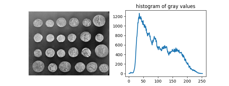
In this example, we will see how to segment objects from a background. We use
the coins image from skimage.data, which shows several coins outlined
against a darker background.
import numpy as np
import matplotlib.pyplot as plt

from skimage import data
from skimage.exposure import histogram

coins = data.coins()
hist, hist_centers = histogram(coins)

fig, axes = plt.subplots(1, 2, figsize=(8, 3))
axes[0].imshow(coins, cmap=plt.cm.gray)
axes[0].axis('off')
axes[1].plot(hist_centers, hist, lw=2)
axes[1].set_title('histogram of gray values')
Text(0.5, 1.0, 'histogram of gray values')
Thresholding
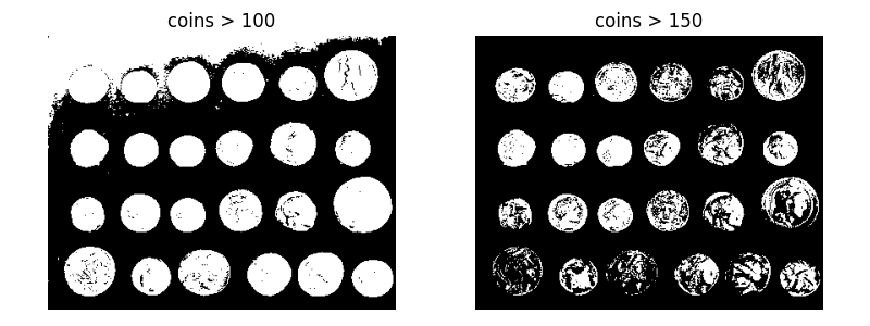
A simple way to segment the coins is to choose a threshold based on the histogram of gray values. Unfortunately, thresholding this image gives a binary image that either misses significant parts of the coins or merges parts of the background with the coins:
fig, axes = plt.subplots(1, 2, figsize=(8, 3), sharey=True)

axes[0].imshow(coins > 100, cmap=plt.cm.gray)
axes[0].set_title('coins > 100')

axes[1].imshow(coins > 150, cmap=plt.cm.gray)
axes[1].set_title('coins > 150')

for a in axes:
    a.axis('off')

plt.tight_layout()
Edge-based segmentation
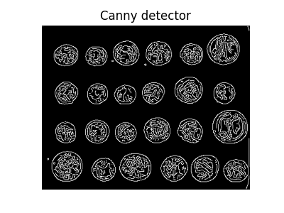
Next, we try to delineate the contours of the coins using edge-based segmentation. To do this, we first get the edges of features using the Canny edge-detector.
from skimage.feature import canny

edges = canny(coins)

fig, ax = plt.subplots(figsize=(4, 3))
ax.imshow(edges, cmap=plt.cm.gray)
ax.set_title('Canny detector')
ax.axis('off')
(-0.5, 383.5, 302.5, -0.5)
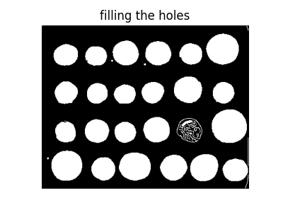
These contours are then filled using mathematical morphology.
from scipy import ndimage as ndi

fill_coins = ndi.binary_fill_holes(edges)

fig, ax = plt.subplots(figsize=(4, 3))
ax.imshow(fill_coins, cmap=plt.cm.gray)
ax.set_title('filling the holes')
ax.axis('off')
(-0.5, 383.5, 302.5, -0.5)
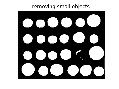
Small spurious objects are easily removed by setting a minimum size for valid objects.
from skimage import morphology

coins_cleaned = morphology.remove_small_objects(fill_coins, 21)

fig, ax = plt.subplots(figsize=(4, 3))
ax.imshow(coins_cleaned, cmap=plt.cm.gray)
ax.set_title('removing small objects')
ax.axis('off')
(-0.5, 383.5, 302.5, -0.5)
However, this method is not very robust, since contours that are not perfectly closed are not filled correctly, as is the case for one unfilled coin above.
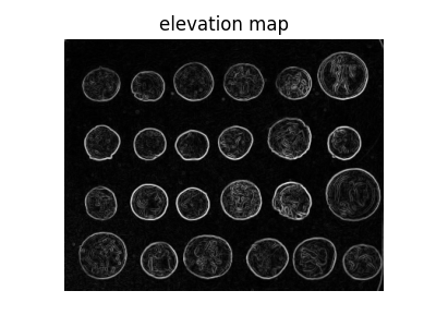
Region-based segmentation
We therefore try a region-based method using the watershed transform. First, we find an elevation map using the Sobel gradient of the image.
from skimage.filters import sobel

elevation_map = sobel(coins)

fig, ax = plt.subplots(figsize=(4, 3))
ax.imshow(elevation_map, cmap=plt.cm.gray)
ax.set_title('elevation map')
ax.axis('off')
(-0.5, 383.5, 302.5, -0.5)
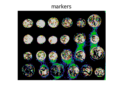
Next we find markers of the background and the coins based on the extreme parts of the histogram of gray values.
markers = np.zeros_like(coins)
markers[coins < 30] = 1
markers[coins > 150] = 2

fig, ax = plt.subplots(figsize=(4, 3))
ax.imshow(markers, cmap=plt.cm.nipy_spectral)
ax.set_title('markers')
ax.axis('off')
(-0.5, 383.5, 302.5, -0.5)
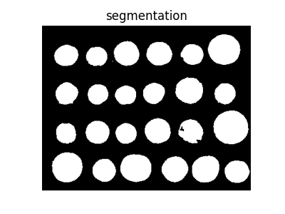
Finally, we use the watershed transform to fill regions of the elevation map starting from the markers determined above:
from skimage import segmentation

segmentation_coins = segmentation.watershed(elevation_map, markers)

fig, ax = plt.subplots(figsize=(4, 3))
ax.imshow(segmentation_coins, cmap=plt.cm.gray)
ax.set_title('segmentation')
ax.axis('off')
(-0.5, 383.5, 302.5, -0.5)
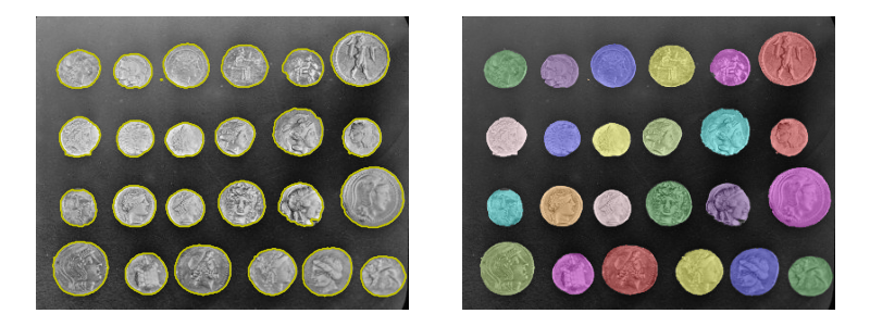
This last method works even better, and the coins can be segmented and labeled individually.
from skimage.color import label2rgb

segmentation_coins = ndi.binary_fill_holes(segmentation_coins - 1)
labeled_coins, _ = ndi.label(segmentation_coins)
image_label_overlay = label2rgb(labeled_coins, image=coins, bg_label=0)

fig, axes = plt.subplots(1, 2, figsize=(8, 3), sharey=True)
axes[0].imshow(coins, cmap=plt.cm.gray)
axes[0].contour(segmentation_coins, [0.5], linewidths=1.2, colors='y')
axes[1].imshow(image_label_overlay)

for a in axes:
    a.axis('off')

plt.tight_layout()

plt.show()
Total running time of the script: ( 0 minutes 0.929 seconds)