Note
Go to the end to download the full example code or to run this example in your browser via Binder.
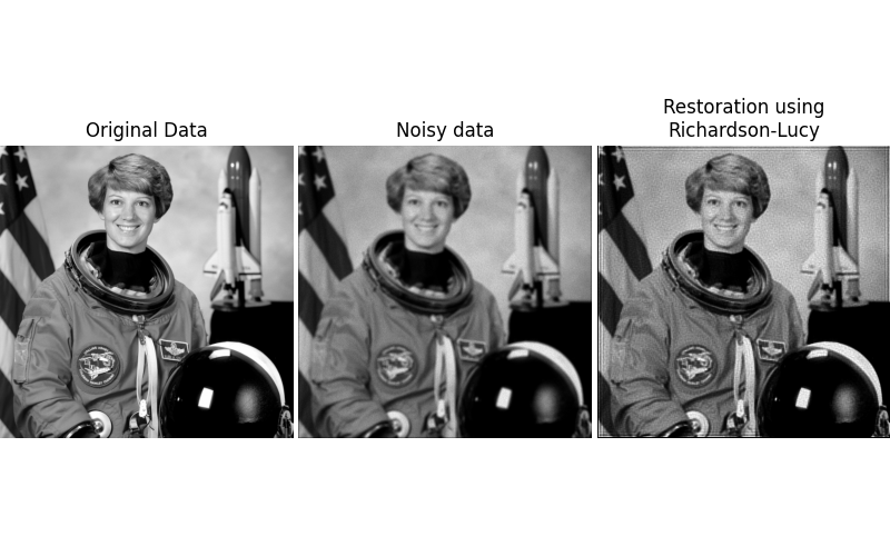
Image Deconvolution#
In this example, we deconvolve an image using the Richardson–Lucy algorithm ([1], [2], [3]).
The algorithm is based on a point spread function (PSF), described as the impulse response of the optical system. The blurred image is sharpened through a number of iterations, which needs to be hand-tuned.
import numpy as np
import matplotlib.pyplot as plt
import skimage as ski

from scipy.signal import convolve2d as conv2


rng = np.random.default_rng()

# Convert astronaut image to grayscale
astro = ski.color.rgb2gray(ski.data.astronaut())

# Define PSF
psf = np.ones((5, 5)) / 25

# Convolve image with the PSF to simulate a blurred image
astro_blurred = conv2(astro, psf, 'same')

# Add Poisson noise to the blurred image (https://en.wikipedia.org/wiki/Shot_noise)
max_photon_count = 1000
astro_noisy = rng.poisson(astro_blurred * max_photon_count) / max_photon_count

# Normalize noisy image
astro_noisy /= np.max(astro_noisy)

# Restore image by means of deconvolution
deconvolved_RL = ski.restoration.richardson_lucy(astro_noisy, psf, num_iter=30)

fig, ax = plt.subplots(ncols=3, figsize=(8, 5))
plt.gray()

for a in (ax[0], ax[1], ax[2]):
    a.axis('off')

ax[0].imshow(astro)
ax[0].set_title('Original Data')

ax[1].imshow(astro_noisy)
ax[1].set_title('Noisy data')

ax[2].imshow(deconvolved_RL)
ax[2].set_title('Restoration using\nRichardson-Lucy')


fig.subplots_adjust(wspace=0.02, hspace=0.2, top=0.9, bottom=0.05, left=0, right=1)
plt.show()
Total running time of the script: (0 minutes 0.602 seconds)