Module: `graph`¶

`skimage.graph.central_pixel`(graph[, nodes, ...])	Find the pixel with the highest closeness centrality.
`skimage.graph.cut_normalized`(labels, rag[, ...])	Perform Normalized Graph cut on the Region Adjacency Graph.
`skimage.graph.cut_threshold`(labels, rag, thresh)	Combine regions separated by weight less than threshold.
`skimage.graph.merge_hierarchical`(labels, ...)	Perform hierarchical merging of a RAG.
`skimage.graph.pixel_graph`(image, *[, mask, ...])	Create an adjacency graph of pixels in an image.
`skimage.graph.rag_boundary`(labels, edge_map)	Comouter RAG based on region boundaries
`skimage.graph.rag_mean_color`(image, labels)	Compute the Region Adjacency Graph using mean colors.
`skimage.graph.route_through_array`(array, ...)	Simple example of how to use the MCP and MCP_Geometric classes.
`skimage.graph.shortest_path`(arr[, reach, ...])	Find the shortest path through an n-d array from one side to another.
`skimage.graph.MCP`(costs[, offsets, ...])	A class for finding the minimum cost path through a given n-d costs array.
`skimage.graph.MCP_Connect`(costs[, offsets, ...])	Connect source points using the distance-weighted minimum cost function.
`skimage.graph.MCP_Flexible`(costs[, offsets, ...])	Find minimum cost paths through an N-d costs array.
`skimage.graph.MCP_Geometric`(costs[, ...])	Find distance-weighted minimum cost paths through an n-d costs array.
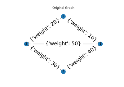
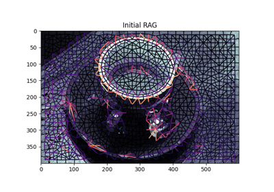
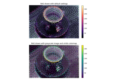
`skimage.graph.RAG`([label_image, ...])	The Region Adjacency Graph (RAG) of an image, subclasses networx.Graph

central_pixel¶

skimage.graph.central_pixel(graph, nodes=None, shape=None, partition_size=100)[source]¶

Find the pixel with the highest closeness centrality.

Closeness centrality is the inverse of the total sum of shortest distances from a node to every other node.

Parameters:

graphscipy.sparse.csr_matrix: The sparse matrix representation of the graph.
nodesarray of int: The raveled index of each node in graph in the image. If not provided, the returned value will be the index in the input graph.
shapetuple of int: The shape of the image in which the nodes are embedded. If provided, the returned coordinates are a NumPy multi-index of the same dimensionality as the input shape. Otherwise, the returned coordinate is the raveled index provided in nodes.
partition_sizeint: This function computes the shortest path distance between every pair of nodes in the graph. This can result in a very large (N*N) matrix. As a simple performance tweak, the distance values are computed in lots of partition_size, resulting in a memory requirement of only partition_size*N.

Returns:

positionint or tuple of int: If shape is given, the coordinate of the central pixel in the image. Otherwise, the raveled index of that pixel.
distancesarray of float: The total sum of distances from each node to each other reachable node.

Examples using `skimage.graph.central_pixel`¶

Use pixel graphs to find an object’s geodesic center

Use pixel graphs to find an object's geodesic center

cut_normalized¶

skimage.graph.cut_normalized(labels, rag, thresh=0.001, num_cuts=10, in_place=True, max_edge=1.0, *, random_state=None)[source]¶

Perform Normalized Graph cut on the Region Adjacency Graph.

Given an image’s labels and its similarity RAG, recursively perform a 2-way normalized cut on it. All nodes belonging to a subgraph that cannot be cut further are assigned a unique label in the output.

Parameters:

labelsndarray

The array of labels.

ragRAG

The region adjacency graph.

threshfloat

The threshold. A subgraph won’t be further subdivided if the value of the N-cut exceeds thresh.

num_cutsint

The number or N-cuts to perform before determining the optimal one.

in_placebool

If set, modifies rag in place. For each node n the function will set a new attribute rag.nodes[n]['ncut label'].

max_edgefloat, optional

The maximum possible value of an edge in the RAG. This corresponds to an edge between identical regions. This is used to put self edges in the RAG.

random_state{None, int, numpy.random.Generator}, optional

If random_state is None the numpy.random.Generator singleton is used. If random_state is an int, a new Generator instance is used, seeded with random_state. If random_state is already a Generator instance then that instance is used.

The random_state is used for the starting point of scipy.sparse.linalg.eigsh.

Returns:

outndarray: The new labeled array.

References

[1]

Shi, J.; Malik, J., “Normalized cuts and image segmentation”, Pattern Analysis and Machine Intelligence, IEEE Transactions on, vol. 22, no. 8, pp. 888-905, August 2000.

Examples

>>> from skimage import data, segmentation, graph
>>> img = data.astronaut()
>>> labels = segmentation.slic(img)
>>> rag = graph.rag_mean_color(img, labels, mode='similarity')
>>> new_labels = graph.cut_normalized(labels, rag)

Examples using `skimage.graph.cut_normalized`¶

Normalized Cut

cut_threshold¶

skimage.graph.cut_threshold(labels, rag, thresh, in_place=True)[source]¶

Combine regions separated by weight less than threshold.

Given an image’s labels and its RAG, output new labels by combining regions whose nodes are separated by a weight less than the given threshold.

Parameters:

labelsndarray: The array of labels.
ragRAG: The region adjacency graph.
threshfloat: The threshold. Regions connected by edges with smaller weights are combined.
in_placebool: If set, modifies rag in place. The function will remove the edges with weights less that thresh. If set to False the function makes a copy of rag before proceeding.

Returns:

outndarray: The new labelled array.

References

[1]

Alain Tremeau and Philippe Colantoni “Regions Adjacency Graph Applied To Color Image Segmentation” DOI:10.1109/83.841950

Examples

>>> from skimage import data, segmentation, graph
>>> img = data.astronaut()
>>> labels = segmentation.slic(img)
>>> rag = graph.rag_mean_color(img, labels)
>>> new_labels = graph.cut_threshold(labels, rag, 10)

Examples using `skimage.graph.cut_threshold`¶

RAG Thresholding

merge_hierarchical¶

skimage.graph.merge_hierarchical(labels, rag, thresh, rag_copy, in_place_merge, merge_func, weight_func)[source]¶

Perform hierarchical merging of a RAG.

Greedily merges the most similar pair of nodes until no edges lower than thresh remain.

Parameters:

labelsndarray: The array of labels.
ragRAG: The Region Adjacency Graph.
threshfloat: Regions connected by an edge with weight smaller than thresh are merged.
rag_copybool: If set, the RAG copied before modifying.
in_place_mergebool: If set, the nodes are merged in place. Otherwise, a new node is created for each merge..
merge_funccallable: This function is called before merging two nodes. For the RAG graph while merging src and dst, it is called as follows merge_func(graph, src, dst).
weight_funccallable: The function to compute the new weights of the nodes adjacent to the merged node. This is directly supplied as the argument weight_func to merge_nodes.

Returns:

outndarray: The new labeled array.

Examples using `skimage.graph.merge_hierarchical`¶

RAG Merging

Hierarchical Merging of Region Boundary RAGs

pixel_graph¶

skimage.graph.pixel_graph(image, *, mask=None, edge_function=None, connectivity=1, spacing=None)[source]¶

Create an adjacency graph of pixels in an image.

Pixels where the mask is True are nodes in the returned graph, and they are connected by edges to their neighbors according to the connectivity parameter. By default, the value of an edge when a mask is given, or when the image is itself the mask, is the euclidean distance between the pixels.

However, if an int- or float-valued image is given with no mask, the value of the edges is the absolute difference in intensity between adjacent pixels, weighted by the euclidean distance.

Parameters:

imagearray: The input image. If the image is of type bool, it will be used as the mask as well.
maskarray of bool: Which pixels to use. If None, the graph for the whole image is used.
edge_functioncallable: A function taking an array of pixel values, and an array of neighbor pixel values, and an array of distances, and returning a value for the edge. If no function is given, the value of an edge is just the distance.
connectivityint: The square connectivity of the pixel neighborhood: the number of orthogonal steps allowed to consider a pixel a neighbor. See scipy.ndimage.generate_binary_structure for details.
spacingtuple of float: The spacing between pixels along each axis.

Returns:

graphscipy.sparse.csr_matrix: A sparse adjacency matrix in which entry (i, j) is 1 if nodes i and j are neighbors, 0 otherwise.
nodesarray of int: The nodes of the graph. These correspond to the raveled indices of the nonzero pixels in the mask.

Examples using `skimage.graph.pixel_graph`¶

Use pixel graphs to find an object’s geodesic center

Use pixel graphs to find an object's geodesic center

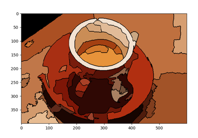
rag_boundary¶

skimage.graph.rag_boundary(labels, edge_map, connectivity=2)[source]¶

Comouter RAG based on region boundaries

Given an image’s initial segmentation and its edge map this method constructs the corresponding Region Adjacency Graph (RAG). Each node in the RAG represents a set of pixels within the image with the same label in labels. The weight between two adjacent regions is the average value in edge_map along their boundary.

labelsndarray: The labelled image.
edge_mapndarray: This should have the same shape as that of labels. For all pixels along the boundary between 2 adjacent regions, the average value of the corresponding pixels in edge_map is the edge weight between them.
connectivityint, optional: Pixels with a squared distance less than connectivity from each other are considered adjacent. It can range from 1 to labels.ndim. Its behavior is the same as connectivity parameter in scipy.ndimage.generate_binary_structure.

Examples

>>> from skimage import data, segmentation, filters, color, graph
>>> img = data.chelsea()
>>> labels = segmentation.slic(img)
>>> edge_map = filters.sobel(color.rgb2gray(img))
>>> rag = graph.rag_boundary(labels, edge_map)

Examples using `skimage.graph.rag_boundary`¶

Region Boundary based RAGs

Hierarchical Merging of Region Boundary RAGs

rag_mean_color¶

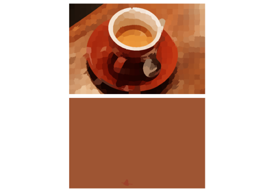
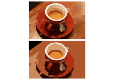
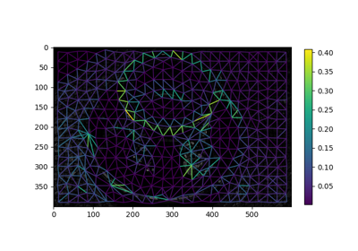
skimage.graph.rag_mean_color(image, labels, connectivity=2, mode='distance', sigma=255.0)[source]¶

Compute the Region Adjacency Graph using mean colors.

Given an image and its initial segmentation, this method constructs the corresponding Region Adjacency Graph (RAG). Each node in the RAG represents a set of pixels within image with the same label in labels. The weight between two adjacent regions represents how similar or dissimilar two regions are depending on the mode parameter.

Parameters:

imagendarray, shape(M, N, […, P,] 3): Input image.
labelsndarray, shape(M, N, […, P]): The labelled image. This should have one dimension less than image. If image has dimensions (M, N, 3) labels should have dimensions (M, N).
connectivityint, optional: Pixels with a squared distance less than connectivity from each other are considered adjacent. It can range from 1 to labels.ndim. Its behavior is the same as connectivity parameter in scipy.ndimage.generate_binary_structure.
mode{‘distance’, ‘similarity’}, optional: The strategy to assign edge weights.

‘distance’ : The weight between two adjacent regions is the \(|c_1 - c_2|\), where \(c_1\) and \(c_2\) are the mean colors of the two regions. It represents the Euclidean distance in their average color.

‘similarity’ : The weight between two adjacent is \(e^{-d^2/sigma}\) where \(d=|c_1 - c_2|\), where \(c_1\) and \(c_2\) are the mean colors of the two regions. It represents how similar two regions are.
sigmafloat, optional: Used for computation when mode is “similarity”. It governs how close to each other two colors should be, for their corresponding edge weight to be significant. A very large value of sigma could make any two colors behave as though they were similar.

Returns:

outRAG: The region adjacency graph.

References

[1]

Alain Tremeau and Philippe Colantoni “Regions Adjacency Graph Applied To Color Image Segmentation” DOI:10.1109/83.841950

Examples

>>> from skimage import data, segmentation, graph
>>> img = data.astronaut()
>>> labels = segmentation.slic(img)
>>> rag = graph.rag_mean_color(img, labels)

Examples using `skimage.graph.rag_mean_color`¶

RAG Thresholding

Normalized Cut

Drawing Region Adjacency Graphs (RAGs)

RAG Merging

route_through_array¶

skimage.graph.route_through_array(array, start, end, fully_connected=True, geometric=True)[source]¶

Simple example of how to use the MCP and MCP_Geometric classes.

See the MCP and MCP_Geometric class documentation for explanation of the path-finding algorithm.

Parameters:

arrayndarray: Array of costs.
startiterable: n-d index into array defining the starting point
enditerable: n-d index into array defining the end point
fully_connectedbool (optional): If True, diagonal moves are permitted, if False, only axial moves.
geometricbool (optional): If True, the MCP_Geometric class is used to calculate costs, if False, the MCP base class is used. See the class documentation for an explanation of the differences between MCP and MCP_Geometric.

Returns:

pathlist: List of n-d index tuples defining the path from start to end.
costfloat: Cost of the path. If geometric is False, the cost of the path is the sum of the values of array along the path. If geometric is True, a finer computation is made (see the documentation of the MCP_Geometric class).

shortest_path¶

skimage.graph.shortest_path(arr, reach=1, axis=-1, output_indexlist=False)[source]¶

Find the shortest path through an n-d array from one side to another.

Parameters:

arrndarray of float64
reachint, optional: By default (reach = 1), the shortest path can only move one row up or down for every step it moves forward (i.e., the path gradient is limited to 1). reach defines the number of elements that can be skipped along each non-axis dimension at each step.
axisint, optional: The axis along which the path must always move forward (default -1)
output_indexlistbool, optional: See return value p for explanation.

Returns:

piterable of int: For each step along axis, the coordinate of the shortest path. If output_indexlist is True, then the path is returned as a list of n-d tuples that index into arr. If False, then the path is returned as an array listing the coordinates of the path along the non-axis dimensions for each step along the axis dimension. That is, p.shape == (arr.shape[axis], arr.ndim-1) except that p is squeezed before returning so if arr.ndim == 2, then p.shape == (arr.shape[axis],)
costfloat: Cost of path. This is the absolute sum of all the differences along the path.

`MCP`¶

class skimage.graph.MCP(costs, offsets=None, fully_connected=True, sampling=None)¶

Bases: object

A class for finding the minimum cost path through a given n-d costs array.

Given an n-d costs array, this class can be used to find the minimum-cost path through that array from any set of points to any other set of points. Basic usage is to initialize the class and call find_costs() with a one or more starting indices (and an optional list of end indices). After that, call traceback() one or more times to find the path from any given end-position to the closest starting index. New paths through the same costs array can be found by calling find_costs() repeatedly.

The cost of a path is calculated simply as the sum of the values of the costs array at each point on the path. The class MCP_Geometric, on the other hand, accounts for the fact that diagonal vs. axial moves are of different lengths, and weights the path cost accordingly.

Array elements with infinite or negative costs will simply be ignored, as will paths whose cumulative cost overflows to infinite.

Parameters:

costsndarray
offsetsiterable, optional: A list of offset tuples: each offset specifies a valid move from a given n-d position. If not provided, offsets corresponding to a singly- or fully-connected n-d neighborhood will be constructed with make_offsets(), using the fully_connected parameter value.
fully_connectedbool, optional: If no offsets are provided, this determines the connectivity of the generated neighborhood. If true, the path may go along diagonals between elements of the costs array; otherwise only axial moves are permitted.
samplingtuple, optional: For each dimension, specifies the distance between two cells/voxels. If not given or None, the distance is assumed unit.

Attributes:

offsetsndarray: Equivalent to the offsets provided to the constructor, or if none were so provided, the offsets created for the requested n-d neighborhood. These are useful for interpreting the traceback array returned by the find_costs() method.

__init__(costs, offsets=None, fully_connected=True, sampling=None)¶: See class documentation.

find_costs()¶

Find the minimum-cost path from the given starting points.

This method finds the minimum-cost path to the specified ending indices from any one of the specified starting indices. If no end positions are given, then the minimum-cost path to every position in the costs array will be found.

Parameters:

startsiterable: A list of n-d starting indices (where n is the dimension of the costs array). The minimum cost path to the closest/cheapest starting point will be found.
endsiterable, optional: A list of n-d ending indices.
find_all_endsbool, optional: If ‘True’ (default), the minimum-cost-path to every specified end-position will be found; otherwise the algorithm will stop when a a path is found to any end-position. (If no ends were specified, then this parameter has no effect.)

Returns:

cumulative_costsndarray: Same shape as the costs array; this array records the minimum cost path from the nearest/cheapest starting index to each index considered. (If ends were specified, not all elements in the array will necessarily be considered: positions not evaluated will have a cumulative cost of inf. If find_all_ends is ‘False’, only one of the specified end-positions will have a finite cumulative cost.)
tracebackndarray: Same shape as the costs array; this array contains the offset to any given index from its predecessor index. The offset indices index into the offsets attribute, which is a array of n-d offsets. In the 2-d case, if offsets[traceback[x, y]] is (-1, -1), that means that the predecessor of [x, y] in the minimum cost path to some start position is [x+1, y+1]. Note that if the offset_index is -1, then the given index was not considered.

goal_reached()¶

int goal_reached(int index, float cumcost) This method is called each iteration after popping an index from the heap, before examining the neighbors.

This method can be overloaded to modify the behavior of the MCP algorithm. An example might be to stop the algorithm when a certain cumulative cost is reached, or when the front is a certain distance away from the seed point.

This method should return 1 if the algorithm should not check the current point’s neighbors and 2 if the algorithm is now done.

offsets¶

traceback(end)¶

Trace a minimum cost path through the pre-calculated traceback array.

This convenience function reconstructs the the minimum cost path to a given end position from one of the starting indices provided to find_costs(), which must have been called previously. This function can be called as many times as desired after find_costs() has been run.

Parameters:

enditerable: An n-d index into the costs array.

Returns:

tracebacklist of n-d tuples: A list of indices into the costs array, starting with one of the start positions passed to find_costs(), and ending with the given end index. These indices specify the minimum-cost path from any given start index to the end index. (The total cost of that path can be read out from the cumulative_costs array returned by find_costs().)

`MCP_Connect`¶

class skimage.graph.MCP_Connect(costs, offsets=None, fully_connected=True)¶

Bases: MCP

Connect source points using the distance-weighted minimum cost function.

A front is grown from each seed point simultaneously, while the origin of the front is tracked as well. When two fronts meet, create_connection() is called. This method must be overloaded to deal with the found edges in a way that is appropriate for the application.

__init__(*args, **kwargs)¶

create_connection()¶

create_connection id1, id2, pos1, pos2, cost1, cost2)

Overload this method to keep track of the connections that are found during MCP processing. Note that a connection with the same ids can be found multiple times (but with different positions and costs).

At the time that this method is called, both points are “frozen” and will not be visited again by the MCP algorithm.

Parameters:

id1int: The seed point id where the first neighbor originated from.
id2int: The seed point id where the second neighbor originated from.
pos1tuple: The index of of the first neighbor in the connection.
pos2tuple: The index of of the second neighbor in the connection.
cost1float: The cumulative cost at pos1.
cost2float: The cumulative costs at pos2.

`MCP_Flexible`¶

class skimage.graph.MCP_Flexible(costs, offsets=None, fully_connected=True)¶

Bases: MCP

Find minimum cost paths through an N-d costs array.

See the documentation for MCP for full details. This class differs from MCP in that several methods can be overloaded (from pure Python) to modify the behavior of the algorithm and/or create custom algorithms based on MCP. Note that goal_reached can also be overloaded in the MCP class.

__init__(costs, offsets=None, fully_connected=True, sampling=None)¶: See class documentation.

examine_neighbor(index, new_index, offset_length)¶

This method is called once for every pair of neighboring nodes, as soon as both nodes are frozen.

This method can be overloaded to obtain information about neighboring nodes, and/or to modify the behavior of the MCP algorithm. One example is the MCP_Connect class, which checks for meeting fronts using this hook.

travel_cost(old_cost, new_cost, offset_length)¶: This method calculates the travel cost for going from the current node to the next. The default implementation returns new_cost. Overload this method to adapt the behaviour of the algorithm.

update_node(index, new_index, offset_length)¶

This method is called when a node is updated, right after new_index is pushed onto the heap and the traceback map is updated.

This method can be overloaded to keep track of other arrays that are used by a specific implementation of the algorithm. For instance the MCP_Connect class uses it to update an id map.

`MCP_Geometric`¶

class skimage.graph.MCP_Geometric(costs, offsets=None, fully_connected=True)¶

Bases: MCP

Find distance-weighted minimum cost paths through an n-d costs array.

See the documentation for MCP for full details. This class differs from MCP in that the cost of a path is not simply the sum of the costs along that path.

This class instead assumes that the costs array contains at each position the “cost” of a unit distance of travel through that position. For example, a move (in 2-d) from (1, 1) to (1, 2) is assumed to originate in the center of the pixel (1, 1) and terminate in the center of (1, 2). The entire move is of distance 1, half through (1, 1) and half through (1, 2); thus the cost of that move is (1/2)*costs[1,1] + (1/2)*costs[1,2].

On the other hand, a move from (1, 1) to (2, 2) is along the diagonal and is sqrt(2) in length. Half of this move is within the pixel (1, 1) and the other half in (2, 2), so the cost of this move is calculated as (sqrt(2)/2)*costs[1,1] + (sqrt(2)/2)*costs[2,2].

These calculations don’t make a lot of sense with offsets of magnitude greater than 1. Use the sampling argument in order to deal with anisotropic data.

__init__(costs, offsets=None, fully_connected=True, sampling=None)¶: See class documentation.

`RAG`¶

class skimage.graph.RAG(label_image=None, connectivity=1, data=None, **attr)[source]¶

Bases: Graph

The Region Adjacency Graph (RAG) of an image, subclasses networx.Graph

Parameters:

label_imagearray of int: An initial segmentation, with each region labeled as a different integer. Every unique value in label_image will correspond to a node in the graph.
connectivityint in {1, …, label_image.ndim}, optional: The connectivity between pixels in label_image. For a 2D image, a connectivity of 1 corresponds to immediate neighbors up, down, left, and right, while a connectivity of 2 also includes diagonal neighbors. See scipy.ndimage.generate_binary_structure.
datanetworkx Graph specification, optional: Initial or additional edges to pass to the NetworkX Graph constructor. See networkx.Graph. Valid edge specifications include edge list (list of tuples), NumPy arrays, and SciPy sparse matrices.
**attrkeyword arguments, optional: Additional attributes to add to the graph.

__init__(label_image=None, connectivity=1, data=None, **attr)[source]¶

Initialize a graph with edges, name, or graph attributes.

Parameters:

incoming_graph_datainput graph (optional, default: None): Data to initialize graph. If None (default) an empty graph is created. The data can be an edge list, or any NetworkX graph object. If the corresponding optional Python packages are installed the data can also be a 2D NumPy array, a SciPy sparse array, or a PyGraphviz graph.
attrkeyword arguments, optional (default= no attributes): Attributes to add to graph as key=value pairs.