Images are numpy arrays¶

Images are represented in scikit-image using standard numpy arrays. This allows maximum inter-operability with other libraries in the scientific Python ecosystem, such as matplotlib and scipy.

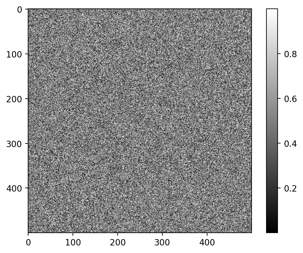
Let’s see how to build a grayscale image as a 2D array:

import numpy as np
from matplotlib import pyplot as plt

random_image = np.random.random([500, 500])

plt.imshow(random_image, cmap='gray')
plt.colorbar();

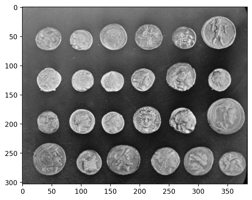
The same holds for “real-world” images:

from skimage import data

coins = data.coins()

print('Type:', type(coins))
print('dtype:', coins.dtype)
print('shape:', coins.shape)

plt.imshow(coins, cmap='gray');

Type: <class 'numpy.ndarray'>
dtype: uint8
shape: (303, 384)

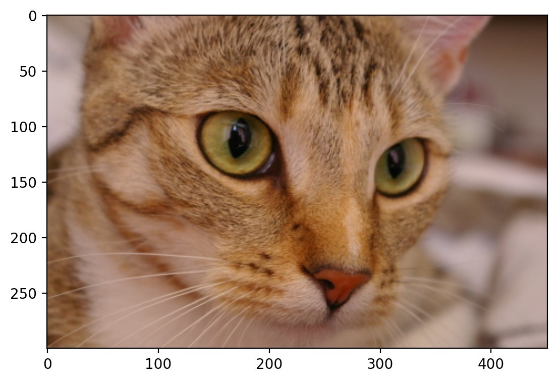
A color image is a 3D array, where the last dimension has size 3 and represents the red, green, and blue channels:

cat = data.chelsea()
print("Shape:", cat.shape)
print("Values min/max:", cat.min(), cat.max())

plt.imshow(cat);

Shape: (300, 451, 3)
Values min/max: 0 231

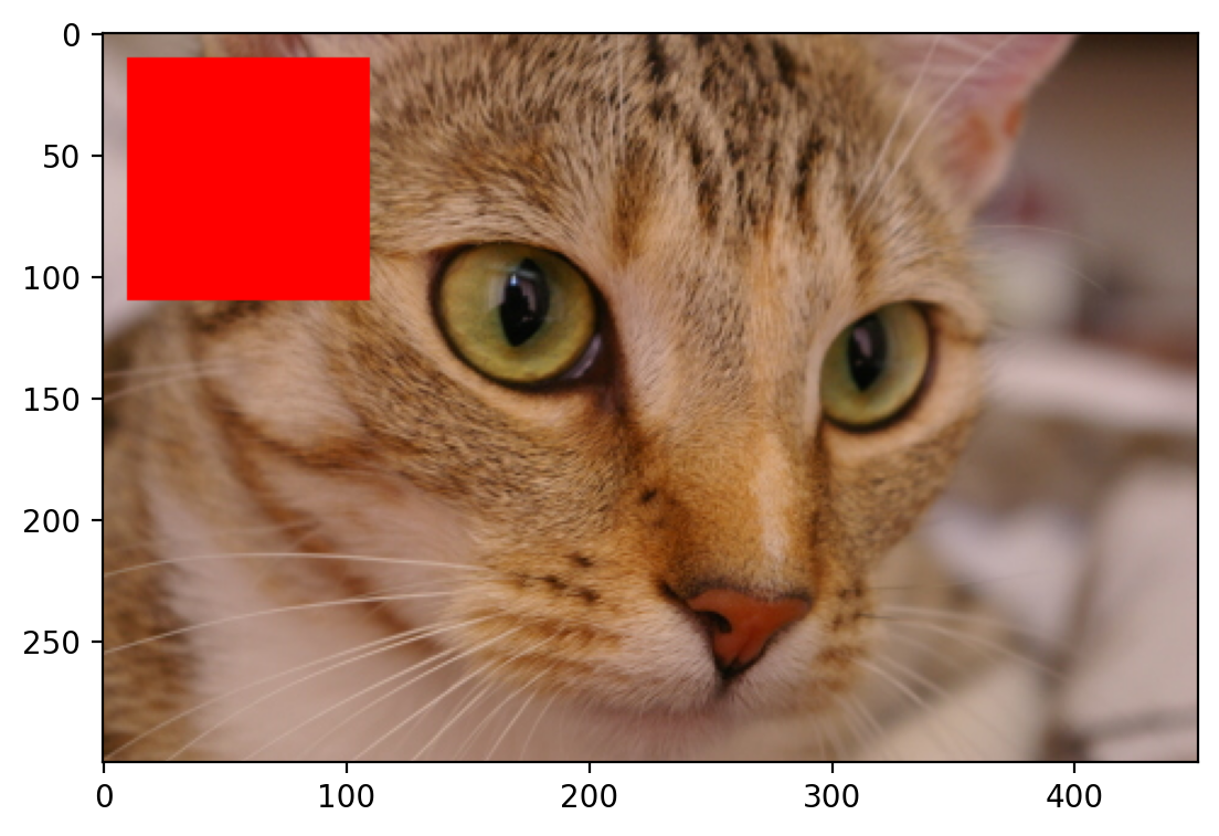
These are just NumPy arrays. E.g., we can make a red square by using standard array slicing and manipulation:

cat[10:110, 10:110, :] = [255, 0, 0]  # [red, green, blue]
plt.imshow(cat);

../_images/00_images_are_arrays_10_0.png

Images can also include transparent regions by adding a 4th dimension, called an alpha layer.

Other shapes, and their meanings¶

Image type	Coordinates
2D grayscale	(row, column)
2D multichannel	(row, column, channel)
3D grayscale (or volumetric)	(plane, row, column)
3D multichannel	(plane, row, column, channel)

Displaying images using matplotlib¶

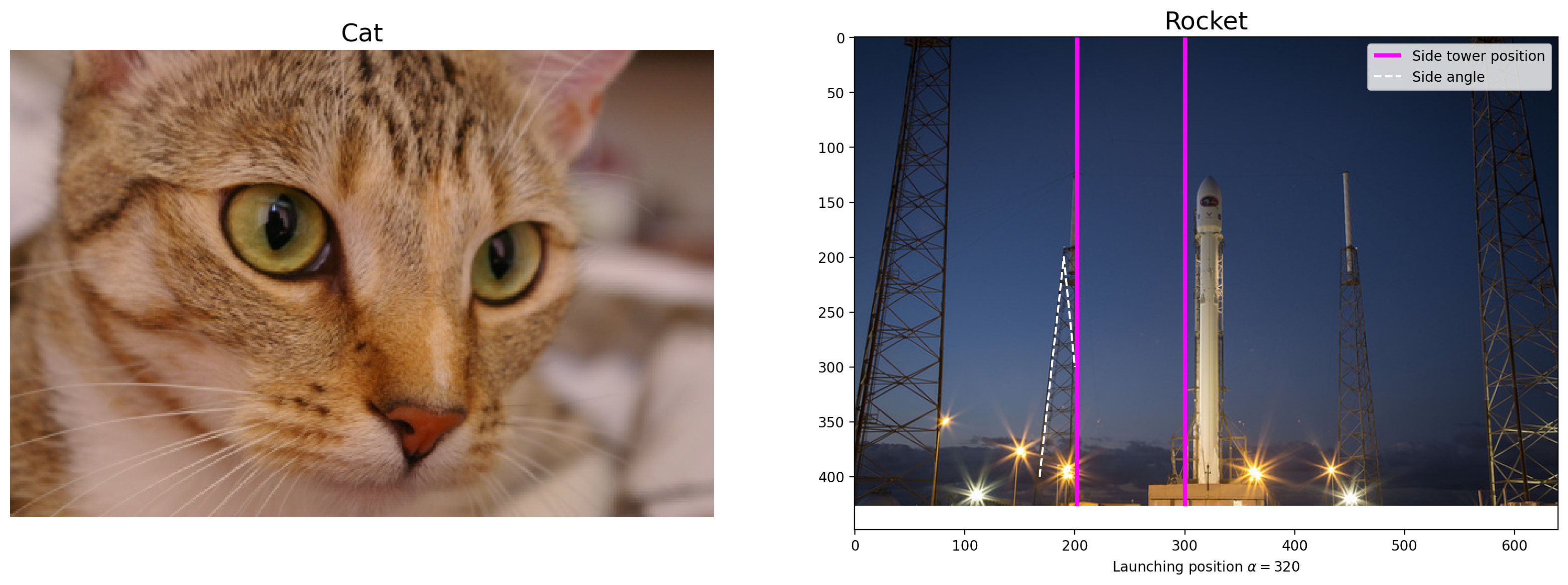
from skimage import data

img0 = data.chelsea()
img1 = data.rocket()

import matplotlib.pyplot as plt

f, (ax0, ax1) = plt.subplots(1, 2, figsize=(20, 10))

ax0.imshow(img0)
ax0.set_title('Cat', fontsize=18)
ax0.axis('off')

ax1.imshow(img1)
ax1.set_title('Rocket', fontsize=18)
ax1.set_xlabel(r'Launching position $\alpha=320$')

ax1.vlines([202, 300], 0, img1.shape[0], colors='magenta', linewidth=3, label='Side tower position')
ax1.plot([168, 190, 200], [400, 200, 300], color='white', linestyle='--', label='Side angle')

ax1.legend();

../_images/00_images_are_arrays_15_0.png

For more on plotting, see the Matplotlib documentation and pyplot API.

Data types and image values¶

In literature, one finds different conventions for representing image values:

  0 - 255   where  0 is black, 255 is white
  0 - 1     where  0 is black, 1 is white

scikit-image supports both conventions–the choice is determined by the data-type of the array.

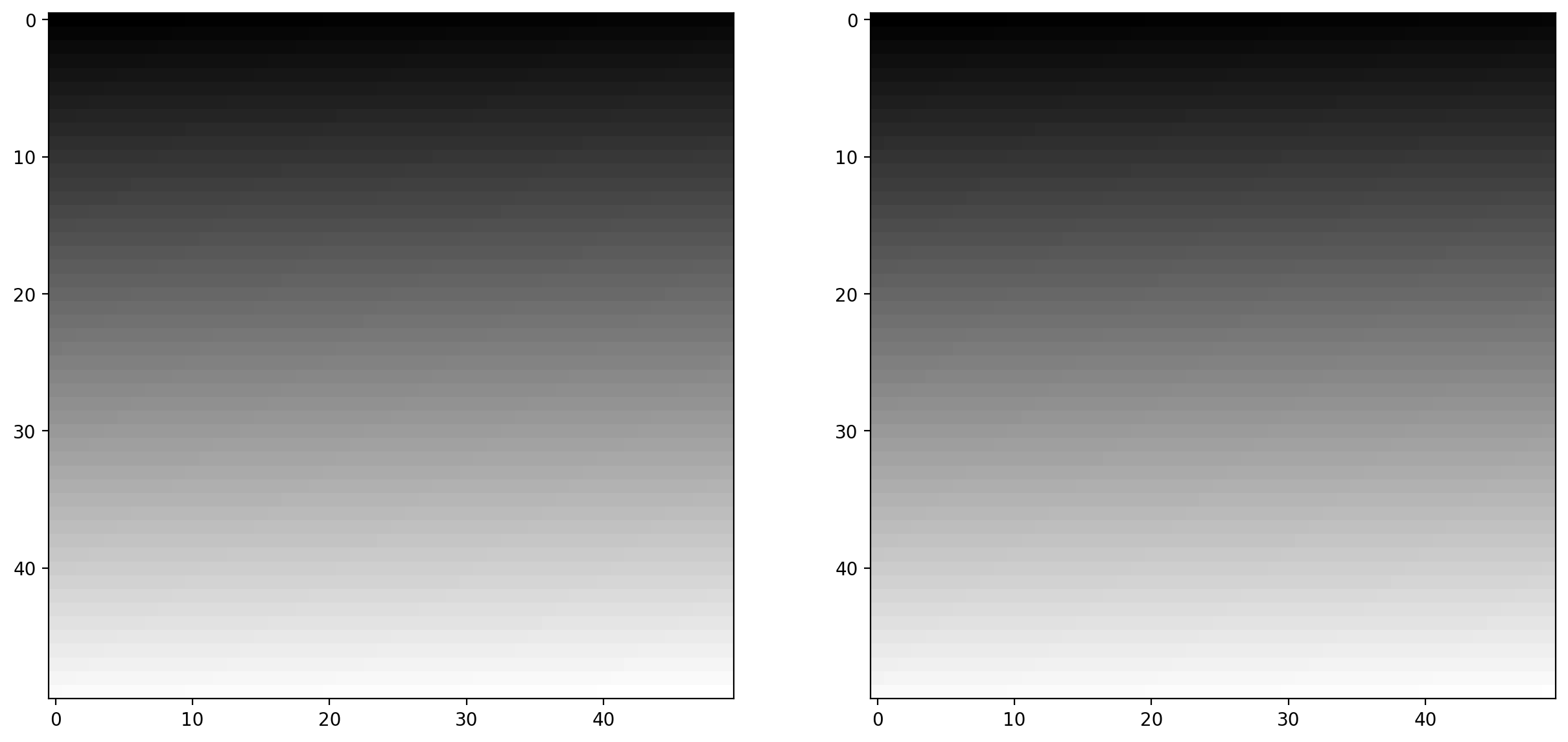
E.g., here, I generate two valid images:

linear0 = np.linspace(0, 1, 2500).reshape((50, 50))
linear1 = np.linspace(0, 255, 2500).reshape((50, 50)).astype(np.uint8)

print("Linear0:", linear0.dtype, linear0.min(), linear0.max())
print("Linear1:", linear1.dtype, linear1.min(), linear1.max())

fig, (ax0, ax1) = plt.subplots(1, 2, figsize=(15, 15))
ax0.imshow(linear0, cmap='gray')
ax1.imshow(linear1, cmap='gray');

Linear0: float64 0.0 1.0
Linear1: uint8 0 255

../_images/00_images_are_arrays_18_1.png

The library is designed in such a way that any data-type is allowed as input, as long as the range is correct (0-1 for floating point images, 0-255 for unsigned bytes, 0-65535 for unsigned 16-bit integers).

You can convert images between different representations by using img_as_float, img_as_ubyte, etc.:

from skimage import img_as_float, img_as_ubyte

image = data.chelsea()

image_ubyte = img_as_ubyte(image)
image_float = img_as_float(image)

print("type, min, max:", image_ubyte.dtype, image_ubyte.min(), image_ubyte.max())
print("type, min, max:", image_float.dtype, image_float.min(), image_float.max())
print()
print("231/255 =", 231/255.)

type, min, max: uint8 0 231
type, min, max: float64 0.0 0.9058823529411765

231/255 = 0.9058823529411765

Your code would then typically look like this:

def my_function(any_image):
   float_image = img_as_float(any_image)
   # Proceed, knowing image is in [0, 1]

We recommend using the floating point representation, given that scikit-image mostly uses that format internally.

Image I/O¶

Mostly, we won’t be using input images from the scikit-image example data sets. Those images are typically stored in JPEG or PNG format. Since scikit-image operates on NumPy arrays, any image reader library that provides arrays will do. Options include imageio, matplotlib, pillow, etc.

scikit-image conveniently wraps many of these in the io submodule, and will use whichever of the libraries mentioned above are installed:

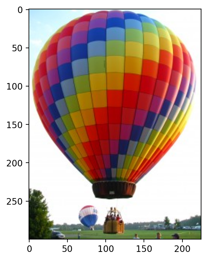
from skimage import io

image = io.imread('../images/balloon.jpg')

print(type(image))
print(image.dtype)
print(image.shape)
print(image.min(), image.max())

plt.imshow(image);

<class 'numpy.ndarray'>
uint8
(300, 225, 3)
0 255

../_images/00_images_are_arrays_24_1.png

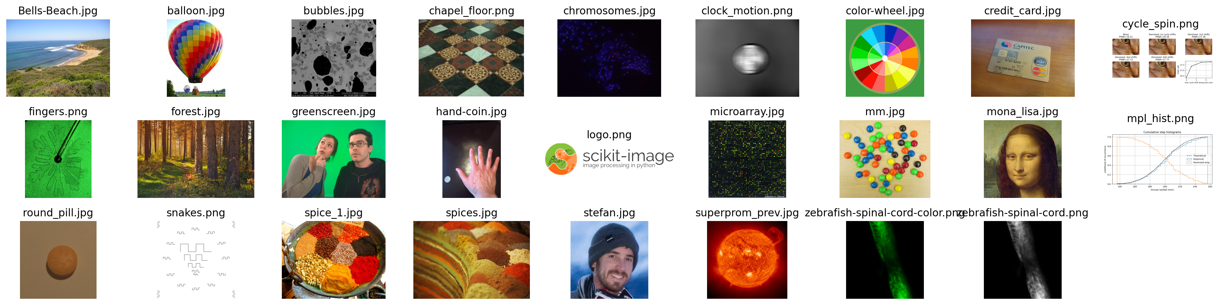
We also have the ability to load multiple images, or multi-layer TIFF images:

ic = io.ImageCollection('../images/*.png:../images/*.jpg')

print('Type:', type(ic))

ic.files

Type: <class 'skimage.io.collection.ImageCollection'>

['../images/Bells-Beach.jpg',
 '../images/balloon.jpg',
 '../images/bubbles.jpg',
 '../images/chapel_floor.png',
 '../images/chromosomes.jpg',
 '../images/clock_motion.png',
 '../images/color-wheel.jpg',
 '../images/credit_card.jpg',
 '../images/cycle_spin.png',
 '../images/fingers.png',
 '../images/forest.jpg',
 '../images/greenscreen.jpg',
 '../images/hand-coin.jpg',
 '../images/logo.png',
 '../images/microarray.jpg',
 '../images/mm.jpg',
 '../images/mona_lisa.jpg',
 '../images/mpl_hist.png',
 '../images/round_pill.jpg',
 '../images/snakes.png',
 '../images/spice_1.jpg',
 '../images/spices.jpg',
 '../images/stefan.jpg',
 '../images/superprom_prev.jpg',
 '../images/zebrafish-spinal-cord-color.png',
 '../images/zebrafish-spinal-cord.png']

import os

f, axes = plt.subplots(nrows=3, ncols=len(ic) // 3 + 1, figsize=(20, 5))

# subplots returns the figure and an array of axes
# we use `axes.ravel()` to turn these into a list
axes = axes.ravel()

for ax in axes:
    ax.axis('off')

for i, image in enumerate(ic):
    axes[i].imshow(image, cmap='gray')
    axes[i].set_title(os.path.basename(ic.files[i]))
    
plt.tight_layout()

../_images/00_images_are_arrays_27_0.png

Aside: `enumerate`¶

enumerate gives us each element in a container, along with its position.

animals = ['cat', 'dog', 'leopard']

for i, animal in enumerate(animals):
    print('The animal in position {} is {}'.format(i, animal))

The animal in position 0 is cat
The animal in position 1 is dog
The animal in position 2 is leopard

Exercise: draw the letter H¶

Define a function that takes as input an RGB image and a pair of coordinates (row, column), and returns a copy with a green letter H overlaid at those coordinates. The coordinates point to the top-left corner of the H.

The arms and strut of the H should have a width of 3 pixels, and the H itself should have a height of 24 pixels and width of 20 pixels.

Start with the following template:

def draw_H(image, coords, color=(0, 255, 0)):
    out = image.copy()
    
    ...
    
    return out 

Test your function like so:

cat = data.chelsea()
cat_H = draw_H(cat, (50, -50))
plt.imshow(cat_H);

Exercise: visualizing RGB channels¶

Display the different color channels of the image along (each as a gray-scale image). Start with the following template:

# --- read in the image ---

image = plt.imread('../images/Bells-Beach.jpg')

# --- assign each color channel to a different variable ---

r = ... # FIXME: grab channel from image...
g = ... # FIXME
b = ... # FIXME

# --- display the image and r, g, b channels ---

f, axes = plt.subplots(1, 4, figsize=(16, 5))

for ax in axes:
    ax.axis('off')

(ax_r, ax_g, ax_b, ax_color) = axes
    
ax_r.imshow(r, cmap='gray')
ax_r.set_title('red channel')

ax_g.imshow(g, cmap='gray')
ax_g.set_title('green channel')

ax_b.imshow(b, cmap='gray')
ax_b.set_title('blue channel')

# --- Here, we stack the R, G, and B layers again
#     to form a color image ---
ax_color.imshow(np.stack([r, g, b], axis=2))
ax_color.set_title('all channels');

Now, take a look at the following R, G, and B channels. How would their combination look? (Write some code to confirm your intuition.)

from skimage import draw

red = np.zeros((300, 300))
green = np.zeros((300, 300))
blue = np.zeros((300, 300))

r, c = draw.circle(100, 100, 100)
red[r, c] = 1

r, c = draw.circle(100, 200, 100)
green[r, c] = 1

r, c = draw.circle(200, 150, 100)
blue[r, c] = 1

f, axes = plt.subplots(1, 3)
for (ax, channel) in zip(axes, [red, green, blue]):
    ax.imshow(channel, cmap='gray')
    ax.axis('off')

<ipython-input-18-4feb18b15cc3>:7: FutureWarning: `draw.circle` is deprecated in favor of `draw.disk`.`draw.circle` will be removed in version 0.19
  r, c = draw.circle(100, 100, 100)
<ipython-input-18-4feb18b15cc3>:10: FutureWarning: `draw.circle` is deprecated in favor of `draw.disk`.`draw.circle` will be removed in version 0.19
  r, c = draw.circle(100, 200, 100)
<ipython-input-18-4feb18b15cc3>:13: FutureWarning: `draw.circle` is deprecated in favor of `draw.disk`.`draw.circle` will be removed in version 0.19
  r, c = draw.circle(200, 150, 100)

../_images/00_images_are_arrays_38_1.png

Exercise: Convert to grayscale (“black and white”)¶

The relative luminance of an image is the intensity of light coming from each point. Different colors contribute differently to the luminance: it’s very hard to have a bright, pure blue, for example. So, starting from an RGB image, the luminance is given by:

\[ Y = 0.2126R + 0.7152G + 0.0722B \]

Use Python 3.5’s matrix multiplication, @, to convert an RGB image to a grayscale luminance image according to the formula above.

Compare your results to that obtained with skimage.color.rgb2gray.

Change the coefficients to 1/3 (i.e., take the mean of the red, green, and blue channels, to see how that approach compares with rgb2gray).

from skimage import color, img_as_float

image = img_as_float(io.imread('../images/balloon.jpg'))

gray = color.rgb2gray(image)
my_gray = ...  # FIXME

# --- display the results ---

f, (ax0, ax1) = plt.subplots(1, 2, figsize=(10, 6))

ax0.imshow(gray, cmap='gray')
ax0.set_title('skimage.color.rgb2gray')

ax1.imshow(my_gray, cmap='gray')
ax1.set_title('my rgb2gray')

Image analysis in Python