Note
Click here to download the full example code or to run this example in your browser via Binder
Inpainting
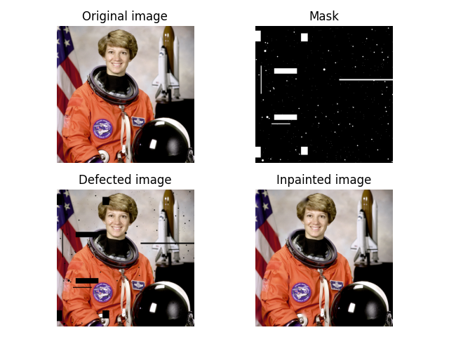
Inpainting [1] is the process of reconstructing lost or deteriorated parts of images and videos.
The reconstruction is supposed to be performed in fully automatic way by exploiting the information presented in non-damaged regions.
In this example, we show how the masked pixels get inpainted by inpainting algorithm based on ‘biharmonic equation’-assumption [2] [3] [4].

import numpy as np
import matplotlib.pyplot as plt

from skimage import data
from skimage.morphology import disk, binary_dilation
from skimage.restoration import inpaint

image_orig = data.astronaut()

# Create mask with six block defect regions
mask = np.zeros(image_orig.shape[:-1], dtype=bool)
mask[20:60, 0:20] = 1
mask[160:180, 70:155] = 1
mask[30:60, 170:195] = 1
mask[-60:-30, 170:195] = 1
mask[-180:-160, 70:155] = 1
mask[-60:-20, 0:20] = 1

# add a few long, narrow defects
mask[200:205, -200:] = 1
mask[150:255, 20:23] = 1
mask[365:368, 60:130] = 1

# add randomly positioned small point-like defects
rstate = np.random.default_rng(0)
for radius in [0, 2, 4]:
    # larger defects are less common
    thresh = 3 + 0.25 * radius  # make larger defects less common
    tmp_mask = rstate.standard_normal(image_orig.shape[:-1]) > thresh
    if radius > 0:
        tmp_mask = binary_dilation(tmp_mask, disk(radius, dtype=bool))
    mask[tmp_mask] = 1

# Apply defect mask to the image over the same region in each color channel
image_defect = image_orig * ~mask[..., np.newaxis]

image_result = inpaint.inpaint_biharmonic(image_defect, mask, channel_axis=-1)

fig, axes = plt.subplots(ncols=2, nrows=2)
ax = axes.ravel()

ax[0].set_title('Original image')
ax[0].imshow(image_orig)

ax[1].set_title('Mask')
ax[1].imshow(mask, cmap=plt.cm.gray)

ax[2].set_title('Defected image')
ax[2].imshow(image_defect)

ax[3].set_title('Inpainted image')
ax[3].imshow(image_result)

for a in ax:
    a.axis('off')

fig.tight_layout()
plt.show()
Total running time of the script: ( 0 minutes 0.215 seconds)

 Source