Note
Go to the end to download the full example code or to run this example in your browser via Binder
Morphological Snakes#
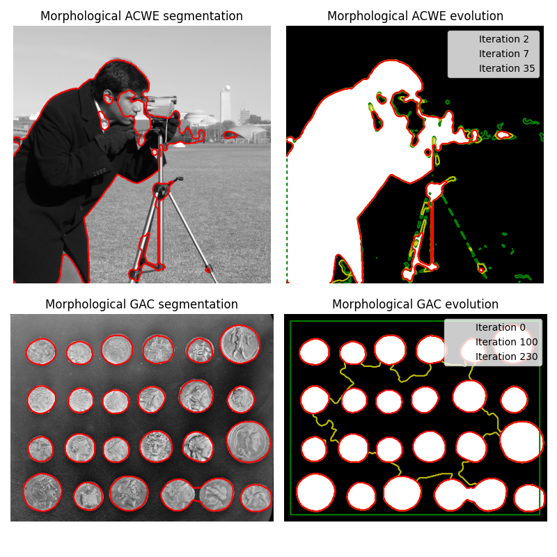
Morphological Snakes [1] are a family of methods for image segmentation. Their behavior is similar to that of active contours (for example, Geodesic Active Contours [2] or Active Contours without Edges [3]). However, Morphological Snakes use morphological operators (such as dilation or erosion) over a binary array instead of solving PDEs over a floating point array, which is the standard approach for active contours. This makes Morphological Snakes faster and numerically more stable than their traditional counterpart.
There are two Morphological Snakes methods available in this implementation:
Morphological Geodesic Active Contours (MorphGAC, implemented in the
function morphological_geodesic_active_contour) and Morphological Active
Contours without Edges (MorphACWE, implemented in the function
morphological_chan_vese).
MorphGAC is suitable for images with visible contours, even when these
contours might be noisy, cluttered, or partially unclear. It requires, however,
that the image is preprocessed to highlight the contours. This can be done
using the function inverse_gaussian_gradient, although the user might want
to define their own version. The quality of the MorphGAC segmentation
depends greatly on this preprocessing step.
On the contrary, MorphACWE works well when the pixel values of the inside and the outside regions of the object to segment have different averages. Unlike MorphGAC, MorphACWE does not require that the contours of the object are well defined, and it works over the original image without any preceding processing. This makes MorphACWE easier to use and tune than MorphGAC.
References#

/home/runner/work/scikit-image/scikit-image/doc/examples/segmentation/plot_morphsnakes.py:95: MatplotlibDeprecationWarning:

The collections attribute was deprecated in Matplotlib 3.8 and will be removed two minor releases later.

/home/runner/work/scikit-image/scikit-image/doc/examples/segmentation/plot_morphsnakes.py:97: MatplotlibDeprecationWarning:

The collections attribute was deprecated in Matplotlib 3.8 and will be removed two minor releases later.

/home/runner/work/scikit-image/scikit-image/doc/examples/segmentation/plot_morphsnakes.py:99: MatplotlibDeprecationWarning:

The collections attribute was deprecated in Matplotlib 3.8 and will be removed two minor releases later.

/home/runner/work/scikit-image/scikit-image/doc/examples/segmentation/plot_morphsnakes.py:133: MatplotlibDeprecationWarning:

The collections attribute was deprecated in Matplotlib 3.8 and will be removed two minor releases later.

/home/runner/work/scikit-image/scikit-image/doc/examples/segmentation/plot_morphsnakes.py:135: MatplotlibDeprecationWarning:

The collections attribute was deprecated in Matplotlib 3.8 and will be removed two minor releases later.

/home/runner/work/scikit-image/scikit-image/doc/examples/segmentation/plot_morphsnakes.py:137: MatplotlibDeprecationWarning:

The collections attribute was deprecated in Matplotlib 3.8 and will be removed two minor releases later.
import numpy as np
import matplotlib.pyplot as plt
from skimage import data, img_as_float
from skimage.segmentation import (
    morphological_chan_vese,
    morphological_geodesic_active_contour,
    inverse_gaussian_gradient,
    checkerboard_level_set,
)


def store_evolution_in(lst):
    """Returns a callback function to store the evolution of the level sets in
    the given list.
    """

    def _store(x):
        lst.append(np.copy(x))

    return _store


# Morphological ACWE
image = img_as_float(data.camera())

# Initial level set
init_ls = checkerboard_level_set(image.shape, 6)
# List with intermediate results for plotting the evolution
evolution = []
callback = store_evolution_in(evolution)
ls = morphological_chan_vese(
    image, num_iter=35, init_level_set=init_ls, smoothing=3, iter_callback=callback
)

fig, axes = plt.subplots(2, 2, figsize=(8, 8))
ax = axes.flatten()

ax[0].imshow(image, cmap="gray")
ax[0].set_axis_off()
ax[0].contour(ls, [0.5], colors='r')
ax[0].set_title("Morphological ACWE segmentation", fontsize=12)

ax[1].imshow(ls, cmap="gray")
ax[1].set_axis_off()
contour = ax[1].contour(evolution[2], [0.5], colors='g')
contour.collections[0].set_label("Iteration 2")
contour = ax[1].contour(evolution[7], [0.5], colors='y')
contour.collections[0].set_label("Iteration 7")
contour = ax[1].contour(evolution[-1], [0.5], colors='r')
contour.collections[0].set_label("Iteration 35")
ax[1].legend(loc="upper right")
title = "Morphological ACWE evolution"
ax[1].set_title(title, fontsize=12)


# Morphological GAC
image = img_as_float(data.coins())
gimage = inverse_gaussian_gradient(image)

# Initial level set
init_ls = np.zeros(image.shape, dtype=np.int8)
init_ls[10:-10, 10:-10] = 1
# List with intermediate results for plotting the evolution
evolution = []
callback = store_evolution_in(evolution)
ls = morphological_geodesic_active_contour(
    gimage,
    num_iter=230,
    init_level_set=init_ls,
    smoothing=1,
    balloon=-1,
    threshold=0.69,
    iter_callback=callback,
)

ax[2].imshow(image, cmap="gray")
ax[2].set_axis_off()
ax[2].contour(ls, [0.5], colors='r')
ax[2].set_title("Morphological GAC segmentation", fontsize=12)

ax[3].imshow(ls, cmap="gray")
ax[3].set_axis_off()
contour = ax[3].contour(evolution[0], [0.5], colors='g')
contour.collections[0].set_label("Iteration 0")
contour = ax[3].contour(evolution[100], [0.5], colors='y')
contour.collections[0].set_label("Iteration 100")
contour = ax[3].contour(evolution[-1], [0.5], colors='r')
contour.collections[0].set_label("Iteration 230")
ax[3].legend(loc="upper right")
title = "Morphological GAC evolution"
ax[3].set_title(title, fontsize=12)

fig.tight_layout()
plt.show()
Total running time of the script: (0 minutes 4.757 seconds)
