9. Image adjustment: transforming image content#
9.1. Color manipulation#
Most functions for manipulating color channels are found in the submodule
skimage.color.
9.1.1. Conversion between color models#
Color images can be represented using different color spaces. One of the most common color spaces is the RGB space, where an image has red, green and blue channels. However, other color models are widely used, such as the HSV color model, where hue, saturation and value are independent channels, or the CMYK model used for printing.
skimage.color provides utility functions to convert images
to and from different color spaces. Integer-type arrays can be
transformed to floating-point type by the conversion operation:
>>> # bright saturated red
>>> red_pixel_rgb = np.array([[[255, 0, 0]]], dtype=np.uint8)
>>> color.rgb2hsv(red_pixel_rgb)
array([[[ 0.,  1.,  1.]]])
>>> # darker saturated blue
>>> dark_blue_pixel_rgb = np.array([[[0, 0, 100]]], dtype=np.uint8)
>>> color.rgb2hsv(dark_blue_pixel_rgb)
array([[[ 0.66666667,  1.        ,  0.39215686]]])
>>> # less saturated pink
>>> pink_pixel_rgb = np.array([[[255, 100, 255]]], dtype=np.uint8)
>>> color.rgb2hsv(pink_pixel_rgb)
array([[[ 0.83333333,  0.60784314,  1.        ]]])
9.1.2. Conversion from RGBA to RGB - Removing alpha channel through alpha blending#
Converting an RGBA image to an RGB image by alpha blending it with a
background is realized with rgba2rgb()
>>> import skimage as ski
>>> img_rgba = ski.data.logo()
>>> img_rgb = ski.color.rgba2rgb(img_rgba)
9.1.3. Conversion between color and gray values#
Converting an RGB image to a grayscale image is realized with
rgb2gray()
>>> img = ski.data.astronaut()
>>> img_gray = ski.color.rgb2gray(img)
rgb2gray() uses a non-uniform weighting of color channels, because of the
different sensitivity of the human eye to different colors. Therefore,
such a weighting ensures luminance preservation
from RGB to grayscale:
>>> red_pixel = np.array([[[255, 0, 0]]], dtype=np.uint8)
>>> ski.color.rgb2gray(red_pixel)
array([[ 0.2125]])
>>> green_pixel = np.array([[[0, 255, 0]]], dtype=np.uint8)
>>> ski.color.rgb2gray(green_pixel)
array([[ 0.7154]])
Converting a grayscale image to RGB with gray2rgb() simply
duplicates the gray values over the three color channels.
9.1.4. Image inversion#
An inverted image is also called complementary image. For binary images, True values
become False and conversely. For grayscale images, pixel values are replaced by the
difference of the maximum value of the data type and the actual value. For RGB
images, the same operation is done for each channel. This operation can be achieved
with skimage.util.invert():
>>> import skimage as ski
>>> img = ski.data.camera()
>>> inverted_img = ski.util.invert(img)
9.1.5. Painting images with labels#
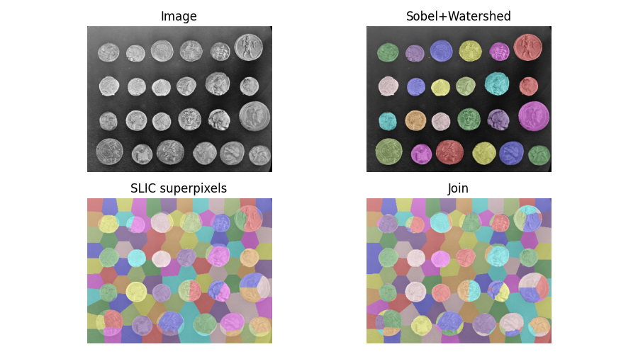
label2rgb() can be used to superimpose colors on a grayscale image
using an array of labels to encode the regions to be represented with the
same color.

9.2. Contrast and exposure#
Image pixels can take values determined by the dtype of the image
(see Image data types and what they mean), such as 0 to 255 for uint8 images or [0,
1] for floating-point images. However, most images either have a
narrower range of values (because of poor contrast), or have most pixel
values concentrated in a subrange of the accessible values.
skimage.exposure provides functions that spread the intensity
values over a larger range.
A first class of methods compute a nonlinear function of the intensity,
that is independent of the pixel values of a specific image. Such methods
are often used for correcting a known non-linearity of sensors, or
receptors such as the human eye. A well-known example is Gamma
correction, implemented
in adjust_gamma().
Other methods re-distribute pixel values according to the histogram of
the image. The histogram of pixel values is computed with
skimage.exposure.histogram():
>>> import numpy as np
>>> import skimage as ski
>>> image = np.array([[1, 3], [1, 1]])
>>> ski.exposure.histogram(image)
(array([3, 0, 1]), array([1, 2, 3]))
histogram() returns the number of pixels for each value bin, and
the centers of the bins. The behavior of histogram() is therefore
slightly different from the one of numpy.histogram(), which returns
the boundaries of the bins.
The simplest contrast enhancement rescale_intensity() consists in
stretching pixel values to the whole allowed range, using a linear
transformation:
>>> import skimage as ski
>>> text = ski.data.text()
>>> text.min(), text.max()
(10, 197)
>>> better_contrast = ski.exposure.rescale_intensity(text)
>>> better_contrast.min(), better_contrast.max()
(0, 255)
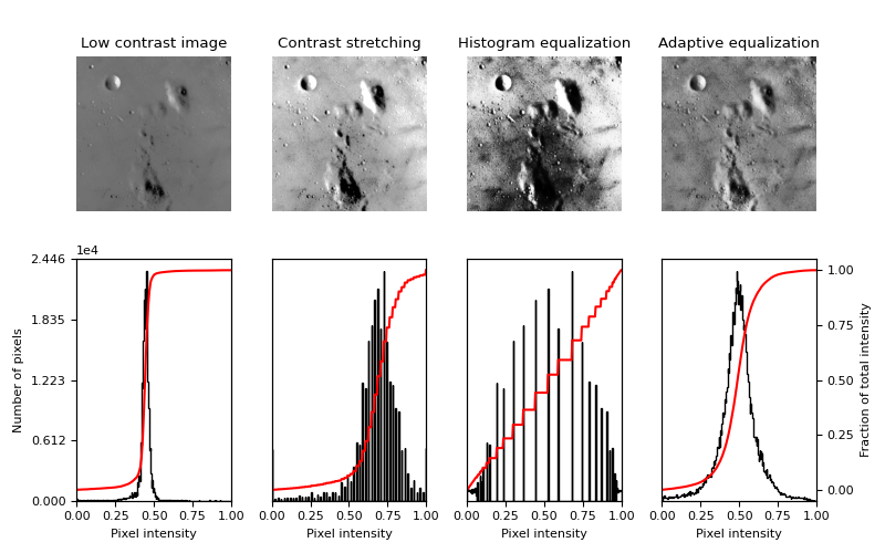
Even if an image uses the whole value range, sometimes there is very little weight at the ends of the value range. In such a case, clipping pixel values using percentiles of the image improves the contrast (at the expense of some loss of information, because some pixels are saturated by this operation):
>>> moon = ski.data.moon()
>>> v_min, v_max = np.percentile(moon, (0.2, 99.8))
>>> v_min, v_max
(10.0, 186.0)
>>> better_contrast = ski.exposure.rescale_intensity(moon, in_range=(v_min, v_max))
The function equalize_hist() maps the cumulative distribution
function (cdf) of pixel values onto a linear cdf, ensuring that all parts
of the value range are equally represented in the image. As a result,
details are enhanced in large regions with poor contrast. As a further
refinement, histogram equalization can be performed in subregions of the
image with equalize_adapthist(), in order to correct for exposure
gradients across the image. See the example
Histogram Equalization.
