Haar-like feature descriptor

Haar-like features are simple digital image features that were introduced in a real-time face detector [1]. These features can be efficiently computed on any scale in constant time, using an integral image [1]. After that, a small number of critical features is selected from this large set of potential features (e.g., using AdaBoost learning algorithm as in [1]). The following example will show the mechanism to build this family of descriptors.

References

[1] (1,2,3)

Viola, Paul, and Michael J. Jones. “Robust real-time face detection.” International journal of computer vision 57.2 (2004): 137-154. https://www.merl.com/publications/docs/TR2004-043.pdf DOI:10.1109/CVPR.2001.990517

import numpy as np
import matplotlib.pyplot as plt

from skimage.feature import haar_like_feature_coord
from skimage.feature import draw_haar_like_feature

Different types of Haar-like feature descriptors

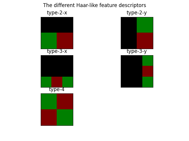
The Haar-like feature descriptors come into 5 different types as illustrated in the figure below. The value of the descriptor is equal to the difference between the sum of intensity values in the green and the red one.

images = [np.zeros((2, 2)), np.zeros((2, 2)),
          np.zeros((3, 3)), np.zeros((3, 3)),
          np.zeros((2, 2))]

feature_types = ['type-2-x', 'type-2-y',
                 'type-3-x', 'type-3-y',
                 'type-4']

fig, axs = plt.subplots(3, 2)
for ax, img, feat_t in zip(np.ravel(axs), images, feature_types):
    coord, _ = haar_like_feature_coord(img.shape[0], img.shape[1], feat_t)
    haar_feature = draw_haar_like_feature(img, 0, 0,
                                          img.shape[0],
                                          img.shape[1],
                                          coord,
                                          max_n_features=1,
                                          random_state=0)
    ax.imshow(haar_feature)
    ax.set_title(feat_t)
    ax.set_xticks([])
    ax.set_yticks([])

fig.suptitle('The different Haar-like feature descriptors')
plt.axis('off')
plt.show()

The value of the descriptor is equal to the difference between the sum of the intensity values in the green rectangle and the red one. The red area is subtracted to the sum of the pixel intensities of the green In practice, the Haar-like features will be placed in all possible location of an image and a feature value will be computed for each of these locations.