Note
Click here to download the full example code or to run this example in your browser via Binder
GLCM Texture Features
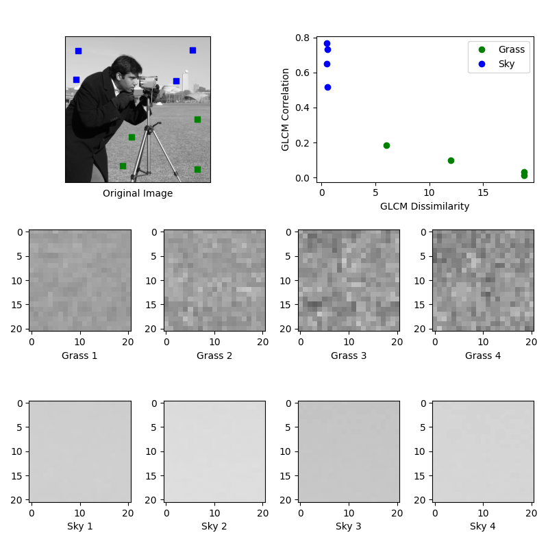
This example illustrates texture classification using gray level co-occurrence matrices (GLCMs) [1]. A GLCM is a histogram of co-occurring grayscale values at a given offset over an image.
In this example, samples of two different textures are extracted from an image: grassy areas and sky areas. For each patch, a GLCM with a horizontal offset of 5 (distance=[5] and angles=[0]) is computed. Next, two features of the GLCM matrices are computed: dissimilarity and correlation. These are plotted to illustrate that the classes form clusters in feature space. In a typical classification problem, the final step (not included in this example) would be to train a classifier, such as logistic regression, to label image patches from new images.
Changed in version 0.19: greymatrix was renamed to graymatrix in 0.19.
Changed in version 0.19: greycoprops was renamed to graycoprops in 0.19.
References

import matplotlib.pyplot as plt

from skimage.feature import graycomatrix, graycoprops
from skimage import data


PATCH_SIZE = 21

# open the camera image
image = data.camera()

# select some patches from grassy areas of the image
grass_locations = [(280, 454), (342, 223), (444, 192), (455, 455)]
grass_patches = []
for loc in grass_locations:
    grass_patches.append(image[loc[0]:loc[0] + PATCH_SIZE,
                               loc[1]:loc[1] + PATCH_SIZE])

# select some patches from sky areas of the image
sky_locations = [(38, 34), (139, 28), (37, 437), (145, 379)]
sky_patches = []
for loc in sky_locations:
    sky_patches.append(image[loc[0]:loc[0] + PATCH_SIZE,
                             loc[1]:loc[1] + PATCH_SIZE])

# compute some GLCM properties each patch
xs = []
ys = []
for patch in (grass_patches + sky_patches):
    glcm = graycomatrix(patch, distances=[5], angles=[0], levels=256,
                        symmetric=True, normed=True)
    xs.append(graycoprops(glcm, 'dissimilarity')[0, 0])
    ys.append(graycoprops(glcm, 'correlation')[0, 0])

# create the figure
fig = plt.figure(figsize=(8, 8))

# display original image with locations of patches
ax = fig.add_subplot(3, 2, 1)
ax.imshow(image, cmap=plt.cm.gray,
          vmin=0, vmax=255)
for (y, x) in grass_locations:
    ax.plot(x + PATCH_SIZE / 2, y + PATCH_SIZE / 2, 'gs')
for (y, x) in sky_locations:
    ax.plot(x + PATCH_SIZE / 2, y + PATCH_SIZE / 2, 'bs')
ax.set_xlabel('Original Image')
ax.set_xticks([])
ax.set_yticks([])
ax.axis('image')

# for each patch, plot (dissimilarity, correlation)
ax = fig.add_subplot(3, 2, 2)
ax.plot(xs[:len(grass_patches)], ys[:len(grass_patches)], 'go',
        label='Grass')
ax.plot(xs[len(grass_patches):], ys[len(grass_patches):], 'bo',
        label='Sky')
ax.set_xlabel('GLCM Dissimilarity')
ax.set_ylabel('GLCM Correlation')
ax.legend()

# display the image patches
for i, patch in enumerate(grass_patches):
    ax = fig.add_subplot(3, len(grass_patches), len(grass_patches)*1 + i + 1)
    ax.imshow(patch, cmap=plt.cm.gray,
              vmin=0, vmax=255)
    ax.set_xlabel(f"Grass {i + 1}")

for i, patch in enumerate(sky_patches):
    ax = fig.add_subplot(3, len(sky_patches), len(sky_patches)*2 + i + 1)
    ax.imshow(patch, cmap=plt.cm.gray,
              vmin=0, vmax=255)
    ax.set_xlabel(f"Sky {i + 1}")


# display the patches and plot
fig.suptitle('Grey level co-occurrence matrix features', fontsize=14, y=1.05)
plt.tight_layout()
plt.show()
Total running time of the script: ( 0 minutes 0.277 seconds)

 Source