Contour finding

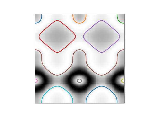
We use a marching squares method to find constant valued contours in an image. In skimage.measure.find_contours, array values are linearly interpolated to provide better precision of the output contours. Contours which intersect the image edge are open; all others are closed.

The marching squares algorithm is a special case of the marching cubes algorithm (Lorensen, William and Harvey E. Cline. Marching Cubes: A High Resolution 3D Surface Construction Algorithm. Computer Graphics SIGGRAPH 87 Proceedings) 21(4) July 1987, p. 163-170).

import numpy as np
import matplotlib.pyplot as plt

from skimage import measure


# Construct some test data
x, y = np.ogrid[-np.pi:np.pi:100j, -np.pi:np.pi:100j]
r = np.sin(np.exp(np.sin(x)**3 + np.cos(y)**2))

# Find contours at a constant value of 0.8
contours = measure.find_contours(r, 0.8)

# Display the image and plot all contours found
fig, ax = plt.subplots()
ax.imshow(r, cmap=plt.cm.gray)

for contour in contours:
    ax.plot(contour[:, 1], contour[:, 0], linewidth=2)

ax.axis('image')
ax.set_xticks([])
ax.set_yticks([])
plt.show()