Local Histogram Equalization

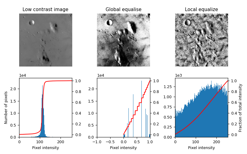
This example enhances an image with low contrast, using a method called local histogram equalization, which spreads out the most frequent intensity values in an image.

The equalized image [1] has a roughly linear cumulative distribution function for each pixel neighborhood.

The local version [2] of the histogram equalization emphasized every local graylevel variations.

These algorithms can be used on both 2D and 3D images.

References

[1]

https://en.wikipedia.org/wiki/Histogram_equalization

[2]

https://en.wikipedia.org/wiki/Adaptive_histogram_equalization

import numpy as np
import matplotlib
import matplotlib.pyplot as plt

from skimage import data
from skimage.util.dtype import dtype_range
from skimage.util import img_as_ubyte
from skimage import exposure
from skimage.morphology import disk
from skimage.morphology import ball
from skimage.filters import rank


matplotlib.rcParams['font.size'] = 9


def plot_img_and_hist(image, axes, bins=256):
    """Plot an image along with its histogram and cumulative histogram.

    """
    ax_img, ax_hist = axes
    ax_cdf = ax_hist.twinx()

    # Display image
    ax_img.imshow(image, cmap=plt.cm.gray)
    ax_img.set_axis_off()

    # Display histogram
    ax_hist.hist(image.ravel(), bins=bins)
    ax_hist.ticklabel_format(axis='y', style='scientific', scilimits=(0, 0))
    ax_hist.set_xlabel('Pixel intensity')

    xmin, xmax = dtype_range[image.dtype.type]
    ax_hist.set_xlim(xmin, xmax)

    # Display cumulative distribution
    img_cdf, bins = exposure.cumulative_distribution(image, bins)
    ax_cdf.plot(bins, img_cdf, 'r')

    return ax_img, ax_hist, ax_cdf


# Load an example image
img = img_as_ubyte(data.moon())

# Global equalize
img_rescale = exposure.equalize_hist(img)

# Equalization
footprint = disk(30)
img_eq = rank.equalize(img, footprint=footprint)


# Display results
fig = plt.figure(figsize=(8, 5))
axes = np.zeros((2, 3), dtype=object)
axes[0, 0] = plt.subplot(2, 3, 1)
axes[0, 1] = plt.subplot(2, 3, 2, sharex=axes[0, 0], sharey=axes[0, 0])
axes[0, 2] = plt.subplot(2, 3, 3, sharex=axes[0, 0], sharey=axes[0, 0])
axes[1, 0] = plt.subplot(2, 3, 4)
axes[1, 1] = plt.subplot(2, 3, 5)
axes[1, 2] = plt.subplot(2, 3, 6)

ax_img, ax_hist, ax_cdf = plot_img_and_hist(img, axes[:, 0])
ax_img.set_title('Low contrast image')
ax_hist.set_ylabel('Number of pixels')

ax_img, ax_hist, ax_cdf = plot_img_and_hist(img_rescale, axes[:, 1])
ax_img.set_title('Global equalise')

ax_img, ax_hist, ax_cdf = plot_img_and_hist(img_eq, axes[:, 2])
ax_img.set_title('Local equalize')
ax_cdf.set_ylabel('Fraction of total intensity')


# prevent overlap of y-axis labels
fig.tight_layout()

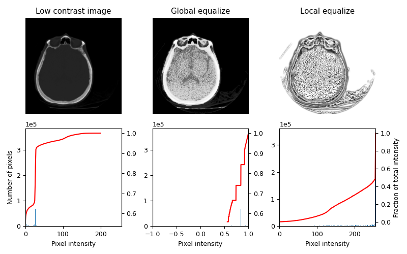
3D Equalization

3D Volumes can also be equalized in a similar fashion. Here the histograms are collected from the entire 3D image, but only a single slice is shown for visual inspection.

matplotlib.rcParams['font.size'] = 9


def plot_img_and_hist(image, axes, bins=256):
    """Plot an image along with its histogram and cumulative histogram.

    """
    ax_img, ax_hist = axes
    ax_cdf = ax_hist.twinx()

    # Display Slice of Image
    ax_img.imshow(image[0], cmap=plt.cm.gray)
    ax_img.set_axis_off()

    # Display histogram
    ax_hist.hist(image.ravel(), bins=bins)
    ax_hist.ticklabel_format(axis='y', style='scientific', scilimits=(0, 0))
    ax_hist.set_xlabel('Pixel intensity')

    xmin, xmax = dtype_range[image.dtype.type]
    ax_hist.set_xlim(xmin, xmax)

    # Display cumulative distribution
    img_cdf, bins = exposure.cumulative_distribution(image, bins)
    ax_cdf.plot(bins, img_cdf, 'r')

    return ax_img, ax_hist, ax_cdf


# Load an example image
img = img_as_ubyte(data.brain())

# Global equalization
img_rescale = exposure.equalize_hist(img)

# Local equalization
neighborhood = ball(3)
img_eq = rank.equalize(img, footprint=neighborhood)

# Display results
fig, axes = plt.subplots(2, 3, figsize=(8, 5))
axes[0, 1] = plt.subplot(2, 3, 2, sharex=axes[0, 0], sharey=axes[0, 0])
axes[0, 2] = plt.subplot(2, 3, 3, sharex=axes[0, 0], sharey=axes[0, 0])

ax_img, ax_hist, ax_cdf = plot_img_and_hist(img, axes[:, 0])
ax_img.set_title('Low contrast image')
ax_hist.set_ylabel('Number of pixels')

ax_img, ax_hist, ax_cdf = plot_img_and_hist(img_rescale, axes[:, 1])
ax_img.set_title('Global equalize')

ax_img, ax_hist, ax_cdf = plot_img_and_hist(img_eq, axes[:, 2])
ax_img.set_title('Local equalize')
ax_cdf.set_ylabel('Fraction of total intensity')


# prevent overlap of y-axis labels
fig.tight_layout()
plt.show()

/home/stefan/src/scikit-image/doc/examples/color_exposure/plot_local_equalize.py:154: MatplotlibDeprecationWarning:

Auto-removal of overlapping axes is deprecated since 3.6 and will be removed two minor releases later; explicitly call ax.remove() as needed.

/home/stefan/src/scikit-image/doc/examples/color_exposure/plot_local_equalize.py:155: MatplotlibDeprecationWarning:

Auto-removal of overlapping axes is deprecated since 3.6 and will be removed two minor releases later; explicitly call ax.remove() as needed.