4. A crash course on NumPy for images#
Images in scikit-image are represented by NumPy ndarrays. Hence, many
common operations can be achieved using standard NumPy methods for
manipulating arrays:
>>> import skimage as ski
>>> camera = ski.data.camera()
>>> type(camera)
<type 'numpy.ndarray'>
Note
Labeled array-like data types, such as
pandas.DataFrame
or xarray.DataArray,
are not natively supported in scikit-image. However, data stored in these types
can be converted to numpy.ndarray with certain assumptions
(see pandas.DataFrame.to_numpy() and xarray.DataArray.data). Particularly,
these conversions ignore the sampling coordinates (DataFrame.index,
DataFrame.columns, or DataArray.coords), which may result in
misrepresented data, for instance, when the original data points are irregularly
spaced.
Retrieving the geometry of the image and the number of pixels:
>>> camera.shape
(512, 512)
>>> camera.size
262144
Retrieving statistical information about image intensity values:
>>> camera.min(), camera.max()
(0, 255)
>>> camera.mean()
118.31400299072266
NumPy arrays representing images can be of different integer or float
numerical types. See Image data types and what they mean for more information about these
types and how scikit-image treats them.
4.1. NumPy indexing#
NumPy indexing can be used both for looking at the pixel values and to modify them:
>>> # Get the value of the pixel at the 10th row and 20th column
>>> camera[10, 20]
153
>>> # Set to black the pixel at the 3rd row and 10th column
>>> camera[3, 10] = 0
Be careful! In NumPy indexing, the first dimension (camera.shape[0])
corresponds to rows, while the second (camera.shape[1]) corresponds
to columns, with the origin (camera[0, 0]) at the top-left corner.
This matches matrix/linear algebra notation, but is in contrast to
Cartesian (x, y) coordinates. See Coordinate conventions below for
more details.
Beyond individual pixels, it is possible to access/modify values of whole sets of pixels using the different indexing capabilities of NumPy.
Slicing:
>>> # Set the first ten lines to "black" (0)
>>> camera[:10] = 0
Masking (indexing with masks of booleans):
>>> mask = camera < 87
>>> # Set to "white" (255) the pixels where mask is True
>>> camera[mask] = 255
Fancy indexing (indexing with sets of indices):
>>> import numpy as np
>>> inds_r = np.arange(len(camera))
>>> inds_c = 4 * inds_r % len(camera)
>>> camera[inds_r, inds_c] = 0
Masks are very useful when you need to select a set of pixels on which to perform the manipulations. The mask can be any boolean array of the same shape as the image (or a shape broadcastable to the image shape). This can be used to define a region of interest, for example, a disk:
>>> nrows, ncols = camera.shape
>>> row, col = np.ogrid[:nrows, :ncols]
>>> cnt_row, cnt_col = nrows / 2, ncols / 2
>>> outer_disk_mask = ((row - cnt_row)**2 + (col - cnt_col)**2 >
...                    (nrows / 2)**2)
>>> camera[outer_disk_mask] = 0
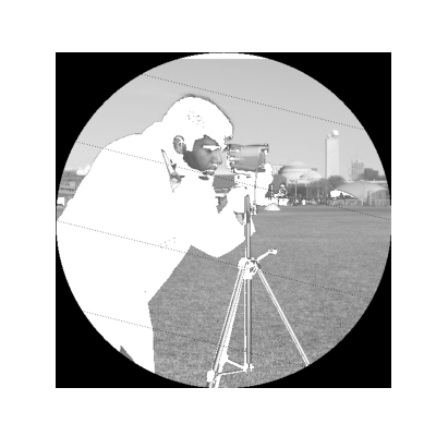
Boolean operations from NumPy can be used to define even more complex masks:
>>> lower_half = row > cnt_row
>>> lower_half_disk = np.logical_and(lower_half, outer_disk_mask)
>>> camera = data.camera()
>>> camera[lower_half_disk] = 0
4.2. Color images#
All of the above remains true for color images. A color image is a NumPy array with an additional trailing dimension for the channels:
>>> cat = ski.data.chelsea()
>>> type(cat)
<type 'numpy.ndarray'>
>>> cat.shape
(300, 451, 3)
This shows that cat is a 300-by-451 pixel image with three channels
(red, green, and blue). As before, we can get and set the pixel values:
>>> cat[10, 20]
array([151, 129, 115], dtype=uint8)
>>> # Set the pixel at (50th row, 60th column) to "black"
>>> cat[50, 60] = 0
>>> # set the pixel at (50th row, 61st column) to "green"
>>> cat[50, 61] = [0, 255, 0]  # [red, green, blue]
We can also use 2D boolean masks for 2D multichannel images, as we did with the grayscale image above:
(Source code, png, hires.png, pdf)
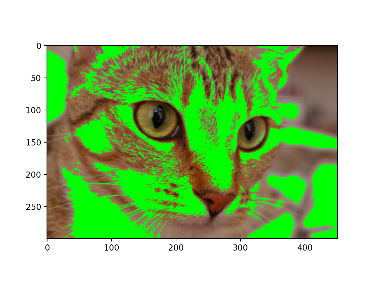
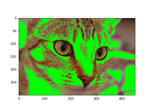
Using a 2D mask on a 2D color image#
The example color images included in skimage.data have channels stored
along the last axis, although other software may follow different conventions.
The scikit-image library functions supporting color images have a
channel_axis argument that can be used to specify which axis of an array
corresponds to channels.
4.3. Coordinate conventions#
Because scikit-image represents images using NumPy arrays, the
coordinate conventions must match. Two-dimensional (2D) grayscale images
(such as camera above) are indexed by rows and columns (abbreviated to
either (row, col) or (r, c)), with the lowest element (0, 0)
at the top-left corner. In various parts of the library, you will
also see rr and cc refer to lists of row and column
coordinates. We distinguish this convention from (x, y), which commonly
denote standard Cartesian coordinates, where x is the horizontal coordinate,
y - the vertical one, and the origin is at the bottom left
(Matplotlib axes, for example, use this convention).
In the case of multichannel images, any dimension (array axis) can be used for
color channels, and is denoted by channel or ch. Prior to scikit-image
0.19, this channel dimension was always last, but in the current release the
channel dimension can be specified by a channel_axis argument. Functions
that require multichannel data default to channel_axis=-1. Otherwise,
functions default to channel_axis=None, indicating that no axis is
assumed to correspond to channels.
Finally, for volumetric (3D) images, such as videos, magnetic resonance imaging
(MRI) scans, confocal microscopy, etc., we refer to the leading dimension
as plane, abbreviated as pln or p.
These conventions are summarized below:
Image type |
Coordinates |
|---|---|
2D grayscale |
(row, col) |
2D multichannel (eg. RGB) |
(row, col, ch) |
3D grayscale |
(pln, row, col) |
3D multichannel |
(pln, row, col, ch) |
Note that the position of ch is controlled by the channel_axis
argument.
Many functions in scikit-image can operate on 3D images directly:
>>> import numpy as np
>>> import scipy as sp
>>> import skimage as ski
>>> rng = np.random.default_rng()
>>> im3d = rng.random((100, 1000, 1000))
>>> seeds = sp.ndimage.label(im3d < 0.1)[0]
>>> ws = ski.segmentation.watershed(im3d, seeds)
In many cases, however, the third spatial dimension has lower resolution
than the other two. Some scikit-image functions provide a spacing
keyword argument to help handle this kind of data:
>>> slics = ski.segmentation.slic(im3d, spacing=[5, 1, 1], channel_axis=None)
Other times, the processing must be done plane-wise. When planes are stacked along the leading dimension (in agreement with our convention), the following syntax can be used:
>>> edges = np.empty_like(im3d)
>>> for pln, image in enumerate(im3d):
...     # Iterate over the leading dimension
...     edges[pln] = ski.filters.sobel(image)
4.4. Notes on the order of array dimensions#
Although the labeling of the axes might seem arbitrary, it can have a significant effect on the speed of operations. This is because modern processors never retrieve just one item from memory, but rather a whole chunk of adjacent items (an operation called prefetching). Therefore, processing of elements that are next to each other in memory is faster than processing them when they are scattered, even if the number of operations is the same:
>>> def in_order_multiply(arr, scalar):
...     for plane in list(range(arr.shape[0])):
...         arr[plane, :, :] *= scalar
...
>>> def out_of_order_multiply(arr, scalar):
...     for plane in list(range(arr.shape[2])):
...         arr[:, :, plane] *= scalar
...
>>> import time
>>> rng = np.random.default_rng()
>>> im3d = rng.random((100, 1024, 1024))
>>> t0 = time.time(); x = in_order_multiply(im3d, 5); t1 = time.time()
>>> print("%.2f seconds" % (t1 - t0))
0.14 seconds
>>> s0 = time.time(); x = out_of_order_multiply(im3d, 5); s1 = time.time()
>>> print("%.2f seconds" % (s1 - s0))
1.18 seconds
>>> print("Speedup: %.1fx" % ((s1 - s0) / (t1 - t0)))
Speedup: 8.6x
When the last/rightmost dimension becomes even larger the speedup is
even more dramatic. It is worth thinking about data locality when
developing algorithms. In particular, scikit-image uses C-contiguous
arrays by default.
When using nested loops, the last/rightmost dimension of the array
should be in the innermost loop of the computation. In the example
above, the *= numpy operator iterates over all remaining dimensions.
4.5. A note on the time dimension#
Although scikit-image does not currently provide functions to
work specifically with time-varying 3D data, its compatibility with
NumPy arrays allows us to work quite naturally with a 5D array of the
shape (t, pln, row, col, ch):
>>> for timepoint in image5d:
...     # Each timepoint is a 3D multichannel image
...     do_something_with(timepoint)
We can then supplement the above table as follows:
Image type |
coordinates |
|---|---|
2D color video |
(t, row, col, ch) |
3D color video |
(t, pln, row, col, ch) |